A Whole New Dimension of Optimization
A Whole New Dimension of Optimization
So far in this series about optimization (1, 2) I've dealt only with univariate objectives . It's time to face the multivariate setting.
Here I'm about to explore two very different approaches that build upon all the previous work. The first will "lift" any univariate method and use it to construct an algorithm for multivariate objectives. The second will generalize the only non-bracketing method encountered thus-far, namely, Newton's method.
Contents
- 1. Coordinatewise Optimization
- 1.1. Sufficient Conditions
- 1.2. Algorithmic Schemes
- 2. Multidimensional Newton's Method
- 2.1. Multidimensional Optimization
- 2.2. Adaptive Steps
- 2.3. Broyden's Method
1. Coordinatewise Optimization
1.1. Sufficient Conditions
It is a dark and stormy night. You're finding yourself all alone in a desolated ally, facing a multivariate objective. All you got is your wallet, your wit and some univariate optimization algorithms you've read about in an obscure blog. Looks like you have only one course of action. But it's insane, desperate and far-fetched. It can never work, can it?
You're in luck! It can, and probably will. As naive as it sounds, optimizing a multivariate objective by operating on each coordinate separably actually often works very well. Moreover, some state-of-the-art machine learning algorithms are based on exactly this concept.
But it does not always work. If it's going to work, we need that a coordinate- wise extrema would be a local extrema. So given an objective $f:R^N\rightarrow R$, and a point $\hat{x}\in R^N$ such that $f(\hat{x}+\delta e_i)\gt f(\hat{x})$ for all small-enough $\delta$ and all $i=1,...,N$ (where $e_i=(0,...,1...,0)\in R^N$ is the standard basis vector) - when does it follow that $f(\hat{x})$ is a local minima of $f$?
Here are 2 simple cases, a positive one and a negative one:
- If $f$ is differentiable, then coordinatewise optimization indeed leads to a candidate extremum (that's easy: $\nabla f(\hat{x})=(\frac{\partial f(\hat{x})}{\partial x_1},...,\frac{\partial f(\hat{x})}{\partial x_N})=0$).
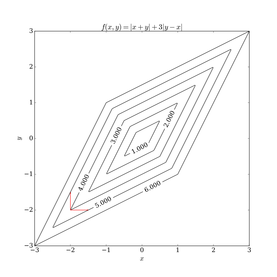
- But if $f$ is not differentiable then coordinatewise optimization doesn't necessarily lead to a candidate extremum, even if it's convex:
A more interesting case comes from mixing the two: consider an objective $f(\vec{x})=g(\vec{x})+\sum_{i=1}^kh_i(x_i)$ where $g$ and the $h_i$s are assumed convex, but only $g$ is surely differentiable.
Note that each term $h_i$ depends only on the $i$-th coordinate. Such functions are called "separable", and such objectives are actually quite common. For example, they can be used to formulate plenty machine-learning algorithms, where $g(x)$ is a differentiable loss-function composed with a parameterization of the hypothesis space, and the $h_i$ functions are regularization terms which are often convex yet non-smooth (as in the case where $\ell_1$ regularization is involved, so $h_i(x)=|x|$ for some $i$s). Similarly, such objectives are also naturally occur in the context of compressed sensing.
And for god is just and merciful, separable objectives can be optimized coordinatewise. Well, maybe it's not so much but about god, as it's about the fact that for any $x\in R^k$ we have - $$ \begin{equation*} \begin{split} f(x)-f(\hat{x})=g(x)-g(\hat{x})+&\sum_{i=1}^k{(h_i(x_i)-h_i(\hat{x}_i))} \ge\nabla g(\hat{x})(x-\hat{x})+\sum_{i=1}^k{(h_i(x_i)-h_i(\hat{x}_i))} \\ & \ge\sum_{i=1}^k{(\underbrace{\nabla_ig(\hat{x})(x_i-\hat{x}_i)+h_i(x_i)-h_i(\hat{x}_i)}_{\ge 0})}\ge 0 \end{split} \end{equation*} $$ where the first inequality follows from the (sub)gradient inequality, and the last inequalities hold since we assumued that $\hat{x}$ is a coordinatewise-minimizer.
1.2. Algorithmic Schemes
The outline of a coordinatewise-optimization algorithm practically writes itself:
- 1. Maintain a "current best solution" $\hat{x}$.
- 2. Repeat until you had enough:
- 2.1. Loop over the coordinates $i=1,...k$:
- 2.1.1. Optimize $f$ as a univariate function of $x_i$ (while holding the other coordinates of $\hat{x}$ fixed).
- 2.1.2. Update the $i$-th coordinate of $\hat{x}$.
This algorithm is guaranteed to convergence (when coordinatewise-optimization is applicable, as discussed in the previous section), and in practice, it usually convergences quickly (though as far as I know, the theoretical reasons for its convergence rate are not yet fully understood).
Still, two issues demand attention: Sweep Patterns and Grouping.
By sweep-patterns I mean the order in which the algorithm goes through the coordinates in each iteration. But first, it should be noted that the fact that the coordinates are optimized sequentially and not in parallel is crucial. In most cases, the following variation will not converge:
- 1. Maintain a "current best solution" $\hat{x}$.
- 2. Repeat until you had enough:
- 2.1. For each coordinates $i=1,...k$, work in parallel:
- 2.1.1. Optimize $f$ as a univariate function of $x_i$.
- 2.2. Update all the coordinates of $\hat{x}$.
In some very special cases it does converge, but even then it tends to converge much slower. For example (though in the very related context of root finding instead of optimization), the Gauss-Seidel algorithm for solving a system of linear equations has the first sequential form while the Jacobi algorithm has the second parallel form. In this special case each algorithm converges if and only if the other one does - but the Gauss-Seidel algorithm is twice as-fast.
For the sequential (and typical) variation, the order in which the coordinates are iterated is often not important, and going over them in a fixed arbitrary order is just fine. But there's a-lot of variation: sometimes the convergence rate may be improved by a randomization of the order; sometimes it's possible to fixate the values of some coordinates and skip their optimization in future iterations; and sometimes the algorithm can access additional information that may hint which coordinates will likely lead to a faster convergence and should be optimized first.
Here's the sequential scheme in pseudo code:
def fix_coordiantes(function, point, free_index):
    point = np.array(point).copy()
    def univariate(x):
        point[free_index] = x
        return function(point)
    return univariate

def coordinatewise_optimization_iteration(objective, initial_argument, univariate_optimizer, sweep_pattern):
    argument = np.array(initial_argument).copy()
    for coordiante in sweep_pattern:
        argument[coordiante] = univariate_optimizer(fix_coordiantes(objective, argument, coordiante))
    return argument


unioptimzer = lambda f: scipy.optimize.minimize_scalar(f, method='Golden').x

def coordinatewise_optimization(objective, initial_argument, max_iterations=100, threshold=1e-6):
    argument, previous_evaluation = initial_argument, objective(initial_argument)
    for iteration in xrange(max_iterations):
        argument = coordinatewise_optimization_iteration(function, argument, unioptimzer, sweep_pattern=[0, 1])
        current_evaluation = function(argument)
        if np.abs(current_evaluation-previous_evaluation)<threshold:
            break
        previous_evaluation = current_evaluation
    return argument, iteration


function = lambda p: p[0]*np.cos(p[1]**2) + 5*p[0]*np.abs(np.sin(p[0]))
minimizer, iterations = coordinatewise_optimization(function, (1.0, 1.0))
assert(np.all([function(minimizer+np.random.normal(0.0, 0.1, 2)) > function(minimizer) for _ in xrange(1000)]))
Finally, the point of "grouping" is that a function $f(x_1,...,x_n):R^n\rightarrow R$ can be treated as a function $f(X_1,...,X_N):R^{n_1}\times R^{n_2}\times...\times R^{n_N}\rightarrow R$ where $\sum_{i=1,...,N}{n_i}=n$, and the scheme above can work by optimizing one group $X_i$ at a time (using some multivariate optimization algorithm for each block). Actually, the degrees of freedom are even greater, since nonadjacent coordinates can be grouped together.
Many times, this can be used to convert problems that are unsuitable for coordinatewise-optimization into problems that are solvable coordinatewise, and lead to significant improvements. For example, it can make a nondifferentiable convex objective into a separable one.
Possibly the most notable example for such a scheme is the SMO algorithm which was one of the earliest efficient optimization methods for SVMs. It minimizes 2-coordinates at the time (though it works in a constraint setting). Nowadays there are better algorithms for learning SVMs, but the state-of-the-art (to my knowledge) is still based on coordinatewise-optimization.
And a concluding note about terminology: many sources (including wikipedia) refer to the algorithmic scheme described here by the name Coordinate Descent. But there's another algorithmic scheme, to be presented in the near future, that also have this name - and I think more deservedly (spoiler: it's a line-search whose search directions are parallel to the axis). So I prefer to reserve the name "Coordinate Descent" for that algorithm, and call the one presented here a "Coordinatewise Optimization".
2. Multidimensional Newton’s Method
2.1. Multidimensional Optimization
Alright, so sometimes it's possible to utilize univariate methods in a multivariate setting without any generalization - simply by applying them coordinate-wise. This can work really great at times, but it doesn't always work. And even when it does, it sometimes doesn't work well.
An alternative approach would be to generalize a univariate method so it would work on "all coordinates at once". A hint as for how it can be done was already given in the previous post where Newton's method for finding roots was introduced, and it was mentioned that it can be used (at least theoretically) for finding roots of multivariate functions.
A quick reminder: Newton method is the iterative algorithm $x_{n+1} \leftarrow x_n + \Delta_n$ where $\Delta_n$ is the solution to the linear system $J(x_n)\Delta_n = -F(x_n)$ for the function of interest $F:R^n\rightarrow R^m$. Ideally, $J(x_n)$ should be computed analytically or algorithmically, but - unlike in the univariate case - it is acceptable to compute it numerically.
The following implementation assumes, for simplicity, $m=n$:
def multivaraite_newton_raphson(F, x0, tolerance_x=None, tolerance_f=None, max_iteartions=50):
    """ Multivaraite Newton-Raphson """
    if tolerance_x is None:
        tolerance_x = default_tolerance(np.min(x0), np.max(x0))
    if tolerance_f is None:
        tolerance_f = tolerance_x

    x = x0
    for iteration in xrange(max_iteartions):
        y, dy = F(x)
        if np.max(np.abs(y)) < tolerance_f:
            break
        delta = np.linalg.solve(dy, -y)
        x = x + delta
        if np.max(np.abs(delta)) < tolerance_x:
            break
    return x, iteration
By courtesy of Fermat's theorem, Newton's method leads to an optimization algorithm which can be efficient for finding candidate extrema points. Naturally, in this context $m=1$ and the objective has the form of $f:R^n\rightarrow R$.
Again, due to Taylor $f(x+h) = f(x) + h^T\nabla f(x) + \frac{1}{2}h^TH(x)h + O(h^3)$. If $h$ leads to an extremum, the optimality condition asserts that $\nabla f(x+h)=0$. Thus differentiation of both sides with respect to $h$ leads to the conclusion that $h$ is the solution of $0\approx\nabla f(x)+H(x)h$ (the equation $H(x)h = -\nabla f(x)$ - or sometimes $\nabla f(x+h) = \nabla f(x) + H(x)h$ - is known as the Secant Equation, and is central to many optimization algorithms).
The iterative scheme of Newton's method is prototypic for many optimization algorithms; each step, the algorithm solves the secant equation $0=\nabla f(x_n)+H(x_n)h$ to obtain a step $h$, which it then takes $x_{n+1}\leftarrow x_n+h$. When - as expected - $x_{n+1}\lt x_n$, the step $h$ is called a "descent step" and its direction is called a descent direction.
This is all fine and dandy, unless you actually want to use this method in practice. That's when constraints regarding time-complexity and memory usage are going to render naive implementations of Newton's method useless. The future posts in this series will deal with actual implementation details of Newton- related optimization algorithms, but for starters let's consider the implementation of Newton's algorithm for multivariate root-finding. This will allow me to introduce more easily some core-ideas that are going to be used over and over again later.
The main themes are the refinement of the concepts of "descent steps" (for which the following section on "Adaptive Steps" serves as an introduction), and approximations for the Jacobian and the Hessian (which will be introduced in the next section, on "Broyden's Method").
2.2. Adaptive Steps
Remember, even though I'm constantly thinking about optimization, here I'm discussing roots. So instead of the extrema of $f:R^n\rightarrow R$, the following will deal with the roots of $F:R^n\rightarrow R^m$.
Given a newton-step $h$, it is not always advised to accept it and set $x_{n+1} \leftarrow x_n + h$. In particular, when $x_n$ is far away from the root, the method may fail completely.
However, a newton-step for $F$ is guaranteed to be a descent direction with respect to $f:=\frac{1}{2}F\cdot F$, thus there exists $0<\lambda\le1$ for which $f(x_n+\lambda h) < f(x_n)$ (yet again a demonstration for the folk wisdom "optimization is easier than finding roots"). Since the minimization of $f$ is a necessary condition for roots of $F$, we use this as a "regularization procedure", and each step becomes $x_{n+1} = x_n + \lambda h$ with $\lambda$ for which $f(x_n+\lambda h)$ has decreased sufficiently.
Furthermore, we require that $f$ will be decreased relatively fast compared to the step-length $\|\lambda h\|$ (specifially, $f(x_{n+1}) < f(x_n) + \alpha\nabla f\cdot (x_{n+1}-x_n)=f(x_n)+\alpha\nabla f\cdot\lambda h$), and that the step-length itself won't be too small (e.g. by imposing a cutoff on $\lambda$).
Following the above improves greatly the global behaviour (far away from the roots) of Newton-Raphson. It remains the decide how to find appropriate $\lambda$. The strategy is to define $g(\lambda):=f(x_n + \lambda h)$, and at each step model it quadratically or cubically based on the known values of $g$ from previous steps, and choose as the next $\lambda$ a value that minimizes $g$'s model (trying to minimize $g$ directly is extremely wasteful in terms of function evaluations).
This is also the core idea behind a major family of optimization algorithms, called line-search algorithms. In details, here:
- Start with $\lambda_0=1$ (a full newton step). Calculate $g(1)=f(x_{n+1})$ and test if $\lambda_0$ is acceptable.
- If it is unacceptable, model $g(\lambda)$ as a quadratic based on $g(0), g'(0), g(1)$ take its minimizer $\lambda_1 = -\frac{g'(0)}{2(g(1))-g(0)-g'(0)}$. Calculate $g(\lambda_1)=f(x_{n+1})$ and test if $\lambda_1$ is acceptable.
- If it is unacceptable, model $g(\lambda)$ as a cubic based on $g(\lambda_{0}), g'(\lambda_{0}), g(\lambda_{k-1}, g(\lambda_{k-2})$ take its minimizer $\lambda_{k} = \frac{-b+\sqrt{b^2-3ag'(0)}}{3a}$ where $(a, b)$ are the coefficients of $g$'s model $g(\lambda) = a\lambda^3 + b\lambda^2 + g'(0)\lambda + g(0)$, so: $$ a = \frac{1}{\lambda_{k-2}-\lambda_{k-1}} \langle\frac{A_2}{\lambda_{k-2}^2}-\frac{A_1}{\lambda_{k-1}^2}\rangle $$ $$ b = \frac{1}{\lambda_{k-2}-\lambda_{k-1}} \langle\frac{A_1\lambda_{k-2}}{\lambda_{k-1}^2}-\frac{A_2\lambda_{k-1}}{\lambda_{k-2}^2}\rangle $$ with $A_i=g(\lambda_{k-i})-g'(0)\lambda_{k-i}-g(0)$.
- Repeat step 3 if necessary, and always enforce $0.1\lambda_1 < \lambda_k < 0.5\lambda_1$.
class AdaptiveSteps(object):
    @staticmethod
    def objective(F, dF):
        """ f := \frac{1}{2}F\cdot F """
        def f(x):
            y = F(x)
            return 0.5*np.dot(y, y)

        def df(x):
            return np.dot(F(x), dF(x))
        return f, df

    @staticmethod
    def line_objective(f, x, newton_step):
        """ g(\lambda):=f(x_n + \lambda h) """
        return lambda length: f(x + length*newton_step)

    @staticmethod
    def is_accepted(previous_image, candidate_image, slope_g, current_length, alpha):
        return candidate_image < previous_image + alpha*slope_g*current_length

    @staticmethod
    def quadratic_based_length(candidate_image, previous_image, slope_g):
        return -slope_g/(2.0*(candidate_image-previous_image-slope_g))

    @staticmethod
    def cubic_based_length(current_length, previous_length, previous_image, candidate_image, previous_candidate_image, slope_g):
        A1 = candidate_image - slope_g*current_length  - previous_image
        A2 = previous_candidate_image - slope_g*previous_length - previous_image
        factor = 1/float(current_length - previous_length)
        a = factor * (A1/(current_length**2) - A2/(previous_length**2))
        b = factor * ((A2*current_length)/(previous_length**2) - (A1*previous_length)/(current_length**2))
        sqrt = np.sqrt(b**2 - 3*a*slope_g)
        if b <= 0:
            return (-b + sqrt)/(3.0*a)
        else:
            return -slope_g/(b + sqrt)

    @staticmethod
    def cutoff(current_length, previous_length):
        if current_length < 0.1*previous_length:
            current_length = 0.1*previous_length
        elif current_length > 0.5*previous_length:
            current_length = 0.5*previous_length
        return current_length
def adaptive_steps_iteration(function, previous_x, previous_value, dy, newton_step, alpha=0.0001, max_iterations=100):
g = AdaptiveSteps.line_objective(function, previous_x, newton_step)
slope = np.dot(dy, newton_step)
candidate_length, candidate_value = 1.0, g(1.0)
if AdaptiveSteps.is_accepted(previous_value, candidate_value, slope, candidate_length, alpha):
return candidate_length, candidate_value
next_candidate_length = AdaptiveSteps.quadratic_based_length(candidate_value, previous_value, slope)
next_candidate_length = AdaptiveSteps.cutoff(next_candidate_length, candidate_length)
previous_candidate_length, candidate_length = candidate_length, next_candidate_length
for iteration in xrange(max_iterations):
previous_candidate_value, candidate_value = candidate_value, g(candidate_length)
if AdaptiveSteps.is_accepted(previous_value, candidate_value, slope, candidate_length, alpha):
break
next_candidate_length = AdaptiveSteps.cubic_based_length(candidate_length, previous_candidate_length,
previous_value, candidate_value, previous_candidate_value, slope)
next_candidate_length = AdaptiveSteps.cutoff(next_candidate_length, candidate_length)
previous_candidate_length, candidate_length = candidate_length, next_candidate_length
return candidate_length, candidate_value
def find_root(F, dF, x0, max_iterations=100):
f, df = AdaptiveSteps.objective(F, dF)
curr_x = x0
prev_y = f(curr_x)
for iteration in xrange(max_iterations):
dy = df(curr_x)
newton_step = np.dot(np.linalg.pinv(dF(curr_x)), -F(curr_x))
length, prev_y = adaptive_steps_iteration(f, curr_x, prev_y, dy, newton_step, alpha=0.0001, max_iterations=10)
curr_x = curr_x + length*newton_step
if np.isclose(prev_y, 0.0):
break
return curr_x, prev_yf1 = lambda x: x[0]**2 + x[1]**2 - 2
df1 = lambda x: np.array([2*x[0], 2*x[1]])
f2 = lambda x: x[0]*x[1]-1
df2 = lambda x: np.array([x[1], x[0]])
F = lambda x: np.array([f1(x), f2(x)])
dF = lambda x: np.vstack((df1(x), df2(x)))
x0 = np.random.normal(0.0, 100, 2)
res_x, res_f = find_root(F, dF, x0, max_iterations=100)
assert(np.allclose(F(res_x), 0.0, atol=1e-4))2.3. Broyden’s Method
Central to Newton-Raphson algorithm, is the equation $J(x_n)\Delta_n = -F(x_n)$ (or the secant equation for optimization). For large problems, the computation of the Jacobian $J(x_n)$ can be expensive. Broyden's method is simply a modification for Newton-Raphson that maintains a cheap approximation for the Jacobian. This idea (here presented in the context of root-finding) is central to the useful BFGS optimization algorithm that will be discussed later.
From the definition of the differential, we know that $J$ is a linear-map that approximately satisfies $J\Delta x = \Delta F$. So at the $i$-th step, Broyden's method approximates $J$ by $J_i$ that solves the equation $J_i(x_{i-1}-x_i) = F_{i-1}-F_i$. Since generally this equation does not determine $J_i$ uniquely, Broyden's method uses $J_{i-1}$ as a prior, and takes as $J_i$ the solution that is closest to $J_{i-1}$ (in the sense of Frobenius norm):
One possible follow-up strategy is to compute a newton step by solving $J(x_n)\Delta_n = -F(x_n)$. Doing this directly has a time complexity of something like $O(N^3)$ (where $N$ is the number of variables). By "something like" I sloppingly mean that solving a system of linear equations in $N$ unknowns has the same (arithmetic) time-complexity as of matrix-multiplication, and specifically, practical applications use matrix factorization algorithms which are $O(N^3)$. But instead of using, say, LU decomposition to find $\Delta_n$ (which takes $\frac{2}{3}N^3$),the Sherman- Morisson inversion formula can be used to obtain -
and the result is an $O(N^2)$ algorithm for approximately find $\Delta_n$.
On the other hand, in order to incorporate adaptive steps (as described above), the approximation for $J_i$ is required (recall: $\nabla(\frac{1}{2}F\cdot F) \approx J^T\cdot F$), while the above method produces an approximation for $J_i^{-1}$. So instead, it's more common to forget all about Sherman-Morisson, and stick to the original iterative approximation of $J_i$.
That's ok, since It's still possible to exploit the fact that in each iteration a 1-rank update is done, and keep the $O(N^2)$ time-complexity, instead of the naive $O(N^3)$. The secret is to solve $J(x_n)\Delta_n = -F(x_n)$ via a QR factorization instead of the (usually preferable) LU factorization. That does the trick, since the QR factorization can be updated iteratively in $O(N^2)$: if $A$ is a $N\times N$ matrix, and $\hat{A}=A+s\otimes t$ (where $s$ and $t$ are in $R^N$), then $A=QR\Rightarrow\hat{A}=Q(R+u\otimes t)$ with $u=Q^Ts$. From here it takes $2(N-1)$ Jacobi rotations in order to obtain a QR factorization of $\hat{A}$.
class Broydens(object):
    def __init__(self, initialX, initialF, initialJ):
        self._prev_x, self._prev_F, self._J = initialX, initialF, initialJ
        self._Q, self._R = scipy.linalg.qr(self._J, pivoting=False)

    def jacobian(self):
        return self._J

    def jacobianQR(self):
        return self._Q, self._R

    def newton_step(self):
        return np.dot(np.linalg.inv(self._R), np.dot(self._Q.T, -self._prev_F))

    def update(self, x, F):
        delta_x = self._prev_x-x
        delta_F = self._prev_F - F

        s, t = delta_F-np.dot(self._J, delta_x), delta_x/np.dot(delta_x, delta_x)
        self._J = self._J  +np.outer(s, t)
        self._Q, self._R = scipy.linalg.qr_update(self._Q, self._R, s, t)
        self._prev_x, self._prev_F = x, F
For example, consider $f(x,y)=[x^2y, 5x+\sin y]$, so $J(x,y)=\begin{bmatrix} 2xy & x^2 \\ 5 & \cos{y} \end{bmatrix}$:
function = lambda p: np.array([p[1]*p[0]**2, 5*p[0]+np.sin(p[1])])
jacobian = lambda p: np.array([[2*p[0]*p[1], p[0]**2],
                               [5, np.cos(p[1])]])
Broyden's approximation is pretty good:
np.random.seed(0)
x0 = np.random.normal(0.0, 5.0, size=2)
broydens = Broydens(x0, function(x0), np.eye(2))

x1 = x0.copy()

for i in xrange(10000):
    x1 = x1 + np.abs(np.random.normal(0.0, 0.0001, size=2))
    broydens.update(x1, function(x1))

np.set_printoptions(precision=3)
print 'Actual Jacobian at x=[%.3f, %.3f]:\n'%(x1[0], x1[1])
print jacobian(x1)
print '\n'
print 'Approximated Jacobian at x=[%.3f, %.3f]:\n'%(x1[0], x1[1])
print broydens.jacobian()
Out:
Actual Jacobian at x=[9.614, 2.785]:
    [[ 53.54   92.42 ]
     [  5.     -0.937]]


Approximated Jacobian at x=[9.614, 2.785]:
    [[ 53.54   92.42 ]
     [  5.     -0.937]]
And it can used to find roots as following:
def broyden_root(objective, initial_x, max_iterations, threshold=1e-6):
    curr_x, curr_y = initial_x, objective(initial_x)
    broydens = Broydens(curr_x, curr_y, np.eye(len(curr_x)))
    for iteration in xrange(max_iterations):
        curr_x = curr_x+broydens.newton_step()
        curr_y = objective(curr_x)
        if np.max(np.abs(curr_y)) < threshold:
            break
        broydens.update(curr_x, curr_y)
    return curr_x, curr_y


x0 = np.random.normal(0, 1, 2)
x1, y1 = broyden_root(function, x0, 50)
print 'Initial point: ', x0
print 'Found root:    ', x1,
print '\t Objective = ', y1
Out:
Initial point:  [ 0.818  0.428]
Found root:     [  6.974e-04   8.168e+01] 	 Objective =  [  3.973e-05   3.425e-08]