The Roots of No Evil
“…nothing at all takes place in the universe in which some rule of maximum or minimum does not appear…” -Leonhard Euler
The above obligatory quote is surely consistent with my experience as an algorithms designer. Optimization problems are not merely "everywhere"; quite literally ALL problems are basically optimization problems, possibly in disguise. This should be enough to convince anyone that optimization is inherently difficult.
But this is a very general argument. What, specifically, makes optimization hard? It's not obvious: after all, given a differentiable function $f:X\rightarrow R$, Fermat's theorem gives an effective necessary condition for optimality ($\nabla f(x_*)=0$), thus it naturally leads to an optimization strategy: numerically solve $\nabla f=0$ by applying a root-finding algorithm to find all the critical points. Moreover, the theorem can be nicely generalized to non-differentiable functions (e.g. in terms of subgradients), and those generalizations are also algorithmically applicable.
So it looks like we're done. Optimization is solved. Hooray!
Time for some party pooping: as it turns out, general optimization is actually easier than general root-finding. I just explained how to solve a difficult problem by reducing it to a harder one.
How come? Well, finding roots requires function inversion, as we're looking for the level-set $f^{-1}(0)$. For general functions, there is very little regularity to exploit, and the best strategy available is essentially following the iterative rule "if the value at the current point is larger than 0, try to find a nearby point with a lower value" (and similarly for values below 0). That's like alternating minimization and maximization steps, so it's at least as hard as optimization.
But things are not all bad. Root-finding is efficiently solvable for univariate functions, and this is the main theme of this post. While the first algorithms to be introduced below will employ root-finding for optimization via Fermat's theorem, it shall quickly become clear that the ideas involved (i.e. bracketing) can be leveraged to design direct optimization algorithms that work for non-smooth and non-convex objective functions (though the objectives can't, of course, behave arbitrarily badly, hence the "no evil" in the title).
This is the first post in a planned series of posts about numerical optimization. The next post will still be limited to univariate objectives, and will focus on differentiable cases. The restriction to univariate objectives is not as limiting as it may seem, since general multidimensional optimization can often be done by solving sequences of a univariate optimization problems. The multivariate setting will be the subject of the following few posts (starting with line-search algorithms), and then I'll write about constrained optimization algorithms, and so on in that fashion until everyone is eaten. I may touch some theoretic-ish issues along the way (e.g. convergence rate, regularity conditions and such) but the focus will always be on the algorithms.
Well, unless I'll give up along the way.
Contents:
- The Bisection Method
- Ridders’ Method (also the false-position and the secant methods)
- Optimization without Roots
- The Golden Section Method
- van Wijngaarden-Dekker-Brent Algorithm
- Differentiable Objectives: A Preview
1. Bisection Method
The general strategy for univariate root-finding is bracketing: maintaining an interval $(a,b)$ such that the signs of $f(a)$ and $f(b)$ differ. When $f:R\rightarrow R$ is continuous, such an interval must contain a root. But this strategy is effective even if $f$ is merely piecewise continuous: then if it doesn't contain a root, it either contains a jump-discontinuity (which numerically is indistinguishable from a root), or the function is unbounded within it (and this is easily detectable).
The simplest bracketing method for root-finding is known as the bisection method. This is a straitforward binary search within the interval:
In [1]:
def bisection(f, interval, tolerance=None):
assert(np.sign(f(interval[0])) != np.sign(f(interval[1])))
interval = [interval[0], interval[1]]
values = [f(interval[0]), f(interval[1])]
if tolerance is None:
tolerance = default_tolerance(interval[0], interval[1])
maxiters = int(np.ceil(np.log2(abs(interval[1]-interval[0])/tolerance)))
for i in xrange(maxiters):
x = interval[0]+(interval[1]-interval[0])*0.5
y = f(x)
if abs(y) < tolerance:
return x, i
elif np.sign(y) == np.sign(values[0]):
interval[0], values[0] = x, y
else:
interval[1], values[1] = x, y
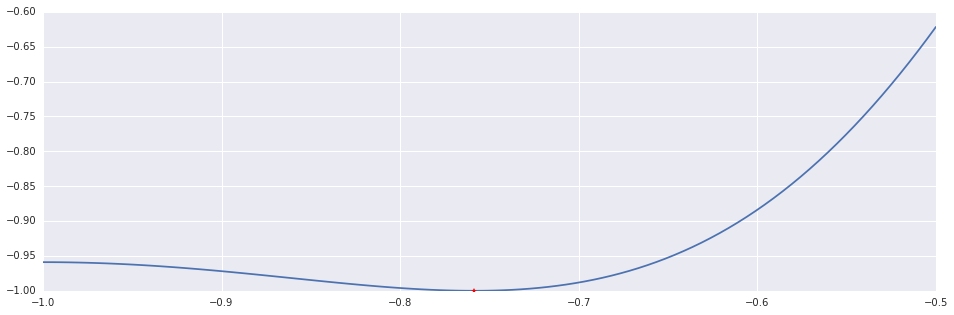
return x, maxitersAs suggested, here's an application of the bisection method to $f'$. To demonstrate all the algorithms in this post, I will use the polynomial $f(x)=x^4+4x^3+x^2-6x+1$ in the interval $(-1, -0.5)$.
Here, differenting $f$ is analytically easy (since it's a polynomial). But this is not generally true. So to keep the flavour of a realistic setting I'm using numerical differentiation (not too realistic though: I'm allowing myself to use first order divided differences).
In [2]:
differentiate = lambda f, delta: lambda x: (f(x+delta)-f(x))/delta

f = lambda x: np.sin(x**4+4*x**3+x**2-6*x+1)
ftag = differentiate(f, 0.00001)
interval_points = np.linspace(-1.0, -0.5, 100)

x, n = bisection(ftag, (-1.0, -0.5))
print 'Bisection Method: %d Iterations.'%n
plt.plot(interval_points, f(interval_points))
plt.plot((x,), (f(x),), 'r*')
Out [2]:
Bisection Method: 37 Iterations.
2. Ridders’ Method
Usually we could do better than a simple binary search, by incorporating some geometrical reasoning into our bracketing method. While this imposes some additional regularity requirements on the objective, it often pays off in terms of convergence rate.
A reasonable first step is to assume local linear-approximability. If $f:R\rightarrow R$ is indeed approximately linear around the bracketing interval, then the root of the linear approximation can be used to contract the interval. This is exactly what both the "false position method" and the "secant method" do. They diverge by how they treat the "approximated root": the secant method always use it to replace the oldest of the two endpoints, while the false position use it to replace the endpoint with the identical sign (unless its sign is 0, of course, which means it's done).
Thus the false position method maintain the foundomental invariant of bracketing (opposite signs for the values at the endpoints), while the secant method may violate it. Both pays a price. On the one hand, the secant method indeed achieves a better convergence rate than bisection when it works, but it may not converge when the linear approximation isn't good enough. On the other hand, the false position is likely to converge, but frequently with no improvement in the convergence rate.
So which one to use? I guess the subtitle above is a spoiler: neither. Use Ridders' method instead.
This is a superlinear (of order $\sqrt{2}$) and "bracket safe" variation of thoes two methods: given an interval $(x_1, x_2)$, denote $x_3=(x_1+x_2)/2$, and replace one of the endpoints (chosen according to the sign) with the new endpoint $x_4 = x_3 + \frac{2(x_3 - x_1)f(x_3)}{\sqrt{f(x_3)^2-f(x_1)f(x_2)}}$.
This expression comes from observing that if the endpoints of $(a,b)$ have opposite signs, then $f(a)-2f(\frac{a+b}{2})Q+f(b)Q^2=0$ has a real positive root $Q_*$, so $(a,f(a)), (\frac{a+b}{2}, f(\frac{a+b}{2})Q), (b,f(b)Q^2)$ falls on a straight line. The result of applying the false-positive method with respect to this lines are satisfactory: $x_4$ is surely within $(x_1, x_2)$, and the convergence rate is quadratic.
In [3]:
def ridders(f, interval, tolerance=None, max_iters=50):
    interval = [interval[0], interval[1]]
    values = [f(interval[0]), f(interval[1])]
    if tolerance is None:
        tolerance = default_tolerance(interval[0], interval[1])

    for i in xrange(max_iters):
        x3 = interval[0]+(interval[1]-interval[0])*0.5
        y3 = f(x3)
        x4 = x3 + (np.sign(values[0]-values[1]))*(x3-interval[0])*y3/np.sqrt(y3**2-values[0]*values[1])
        y4 = f(x4)
        if abs(y4) < tolerance:
            return x4, i
        elif np.sign(y4) == np.sign(values[0]):
            interval[0], values[0] = x4, y4
            if np.sign(y3) == np.sign(values[1]):
                interval[1], values[1] = x3, y3
        else:
            interval[1], values[1] = x4, y4
            if np.sign(y3) == np.sign(values[0]):
                interval[0], values[0] = x3, y3
    return x4, max_iters
In [4]:
x, n = ridders(ftag, (-1.0, -0.5))
print "Ridder's Method: %d Iterations."%n
plt.plot(interval_points, f(interval_points))
plt.plot((x,), (f(x),), 'r*')
Out [4]:
Ridder's Method: 6 Iterations.

3. Optimization without Roots
So the general strategy seems to be working. But so far we conveniently ignored some major problems. For starters, the verb "to optimize" obfuscates the fact that in each case, we're interested in specifically minimization or specifically maximization. Yet, looking for a stationary point $f'(x_*)=0$ could lead to either. The above algorithms can not distinguish minima from maxima.
Fixing it requires constantly querying for the values of $f$, not just $f'$. But function evaluations could very well be (and usually are) the most expensive steps in the algorithm, so it is a costly fix. Moreover, it'd still leave us with another problem: multiple roots and very close roots.
These create a problem for bracketing, since then a small interval $(a,b)$ may contain a root while $\mathrm{sign}f(a)=\mathrm{sign}f(b)$. Again, there are ways to mitigate this issue. But there's a better approach, which nullify those problems all together and has an additional major advantage.
As mentioned above, root-finding is not easier than optimization - and surprisingly this fact has some positive consequences. The idea of bracketing, underlying pretty much all the univariate root-finding methods (with one notable exception, to be discussed later), could be modified slightly and be used for optimizing $f:R\rightarrow R$ directly, instead of for solving $f'=0$.
The major advantage is that those modifications also work very well for non- differentiable functions, but even more importantly, they don't require a computation of the derivative. This is good because generally, even when the objective is differentiable, its gradient may not be easily available. So it's desirable to devise methods that require nothing more than evaluations of the objective.
The idea is to maintain triplets of points $(a,b,c)$, not just pairs $(a,b)$, and instead of the invariant $\mathrm{sign}f(a)=\mathrm{sign}f(b)$, enforce $f(b)\lt\min{(f(a),f(c))}$ (which implies that $f$ has a minimum in $(a,c)$).
4. Golden Section Method
Such a modification, applied to the bisection method, leads to the golden section method. Now we have a triplet $(a,b,c)$, not a pair $(a,b)$, so the meaning of "binary search" is not immediately clear. But it's obvious we must choose either $b'\in(a,b)$ or $b'\in(b,c)$, and it's sensible to be conservative about it.
Say we test $b'\in(a,b)$. Then afterwards the triplet would be either $(a,b',b)$ or $(b',b,c)$. Being conservative means to make a choice for which $|b-a|=|c-b'|$ (since otherwise, the new interval might be "larger than necessary"). That's how the "golden section" method got its name: this strategy implies that the ratio of the two halfs $(a,b)$ and $(b,c)$ is invariant. and equal to $\phi\approx 1.618033$.
In [6]:
def golden_section(f, triplet, tolerance, maxiters=50):
    golden = scipy.constants.golden - 1.0

    triplet = [triplet[0], triplet[1], triplet[2]]
    values = [f(triplet[0]), f(triplet[1]), f(triplet[2])]
    assert(values[1] < min(values[0], values[2]))

    maxiters = int(np.ceil(np.log2(abs(triplet[2]-triplet[0])/tolerance)))

    for i in xrange(maxiters):
        if (triplet[2]-triplet[0]) < tolerance*np.abs(values[1]):
            return triplet[1], i
        if (triplet[1]-triplet[0]) > (triplet[2]-triplet[1]):
            x = triplet[0]+golden*(triplet[1]-triplet[0])
            y = f(x)
            if y < values[1]:
                triplet, values = [triplet[0], x, triplet[1]], [values[0], y, values[1]]
            else:
                triplet, values = [x, triplet[1], triplet[2]], [y, values[1], values[2]]
        else:
            x = triplet[1]+golden*(triplet[2]-triplet[1])
            y = f(x)
            if y < values[1]:
                triplet, values = [triplet[1], x, triplet[2]], [values[1], y, values[2]]
            else:
                triplet, values = [triplet[0], triplet[1], x], [values[0], values[1], y]
    return triplet[1], maxiters
Here’s a demonstration. Note how the derivative is not used.
In [7]:
x, n = golden_section(f=f, triplet=(-1.0, -0.9, 0.0), tolerance=1e-6, maxiters=50)
print "Golden Section: %d Iterations."%n
plt.plot(interval_points, f(interval_points))
plt.plot((x,), (f(x),), 'r*')
Out [7]:
Golden Section: 20 Iterations.

5. van Wijngaarden-Dekker-Brent Method
Applying this modification to Ridder's method doesn't seem too promising. Following the assumption that the objective is approximately locally linear leads to the conclusion that the extremal points are on the interval's boundary. In other words, it leads nowhere.
Continuing with the idea of geometrical approximation, the next natural step is to go from linear functions to quadratic functions. This requires maintaining 3 points, and not just 2 - which may seem a bit awkward in the context of root- finding, but is the default anyway when using bracketing for optimization.
Brent's method uses $(x_i,y_i)_{i=1,2,3}$, to perform at each step an inverse quadratic interpolation $x=f(y)$ (with $f(y)=\alpha y^2+\beta y+\gamma$), and improve the bracketing using $f(0)$. The next root-approximation is then $x=b+\frac{P}{Q}$ for $P=S[T(R-T)(c-b)-(1-R)(b-a)]$ and $Q=(T-1)(R-1)(S-1)$, with $R:=\frac{f(b)}{f(c)}$, $S:=\frac{f(b)}{f(a)}$ and $T:=\frac{f(a)}{f(c)}$.
The case of colinear points requires some special treatment, since in this case, of course, quadratic interpolation is infeasible. This is mitigated by the algorithm by turning to linear approximation, and performing a step using the secant method. As discussed above, the secant method converges fast when the objective is well-behaved, but it may fail when it isn't.
It is pointless to use another - safer - method instead in the degenerated case, since the quadratic interpolation is prone to the same behaviour. Instead, this method is optimistic. It assumes well-behaviour, and acts optimally under this assumption. At the same time, it's also careful. Each step this assumption is tested, and when it does not hold - the algorithm falls back to a bisection step - which might be rather slow - but its convergence is guaranteed.
Here's this algorithm for root-finding:
In [8]:
def brent(f, interval, tolerance=None, maxiters=50):
    x_counter, x_curr_root = interval[0], interval[1]
    y_counter, y_curr_root = f(x_counter), f(x_curr_root)


    if tolerance is None:
        tolerance = default_tolerance(x_curr_root, x_counter)
    bisection_flag = False

    def secant_step():
        return x_curr_root - y_curr_root*(x_curr_root-x_counter)/(y_curr_root-y_counter)

    def quadratic_step():
        R = y_curr_root/y_prev_root
        S = y_prev_root/y_counter
        T = y_counter/y_prev_root
        P = S*(T*(R-T)*(x_prev_root-x_curr_root)-(1-R)*(x_curr_root-x_counter))
        Q = (T-1)*(R-1)*(S-1)
        return x_curr_root + P/Q

    def interpolation_step():
        if (x_prev_root != x_curr_root) and (x_counter != x_curr_root) and (x_counter != x_prev_root):
            return quadratic_step()
        return secant_step()

    def bisection_step():
        return x_counter + (x_curr_root-x_counter)*0.5


    def reject_interpolation(s):
        dp = (3*x_counter + x_curr_root)/4.0
        if dp < x_curr_root:
            flag = (s < dp) or (s > x_curr_root)
        else:
            flag = (s < x_curr_root) or (s > dp)
        return flag

    def slow_shrinkage(s):
        if np.isclose(x_curr_root, x_prev_root):
            return False
        if bisection_flag:
            flag = (abs(s-x_curr_root) >= abs(x_curr_root-x_prev_root)*0.5)
        else:
            flag = (abs(s-x_curr_root) >= abs(x_prev_root-x_prev_prev_root)*0.5)
        return flag

    def slow_convergence(tol):
        if np.isclose(x_curr_root, x_prev_root):
            return False
        if bisection_flag:
            flag = abs(x_curr_root-x_prev_root) < tol
        else:
            flag = abs(x_prev_root-x_prev_prev_root) < tol
        return flag


    if abs(y_counter) < abs(y_curr_root):
        x_counter, x_curr_root = x_curr_root, x_counter
        y_counter, y_curr_root = y_curr_root, y_counter
    x_prev_root, y_prev_root = x_counter, y_counter
    x_prev_prev_root = x_curr_root

    for i in xrange(maxiters):
        if abs(y_curr_root) < tolerance:
            return x_curr_root, i
        convergence_tolerance = 2.0*abs(x_curr_root)*np.finfo(np.float64).eps + 0.5*tolerance

        x_next = interpolation_step()
        bisection_flag = reject_interpolation(x_next) or slow_shrinkage(x_next) or slow_convergence(convergence_tolerance)
        if bisection_flag:
            x_next = bisection_step()
        y_next = f(x_next)

        x_prev_prev_root = x_prev_root
        x_prev_root, y_prev_root = x_curr_root, y_curr_root

        if np.sign(y_next) != np.sign(y_counter):
            x_curr_root, y_curr_root = x_next, y_next
        else:
            x_counter, y_counter = x_next, y_next

        if abs(y_counter) < abs(y_curr_root):
            x_counter, x_curr_root = x_curr_root, x_counter
            y_counter, y_curr_root = y_curr_root, y_counter

    return x_curr_root, maxiters
To modify it for direct optimization is rather simple, and the result works well.
Now, instead of solving $f(x)=0$ (which was done by performing an inverse interpolation, and its value at 0) - we optimize the quadratic functions. This is analytically easy: $x_*=-\frac{\beta}{2\alpha}$, or in terms of the triplet $ x_*=x_1-\frac{1}{2}\frac{(x_1-x_0)^2(y_1-y_2)-(x_1-x_2)^2(y_1-y_0)}{(x_1-x_0)(y_ 1-y_2)-(x_1-x_2)(y_1-y_0)}$, and instead of falling back on the bisection method, we fall back on the golden section method.
In [9]:
def brent_opt(f, triplet, tolerance, maxiters=50):
    golden = scipy.constants.golden - 1.0

    triplet = [triplet[0], triplet[1], triplet[2]]
    values = [f(triplet[0]), f(triplet[1]), f(triplet[2])]
    assert(values[1] < min(values[0], values[2]))
    ref_step = 0.0

    def interpolation_step():
        A = triplet[1]-triplet[0]
        B = triplet[1]-triplet[2]
        C = values[1]-values[2]
        D = values[1]-values[0]
        X = A*C
        Y = B*D
        step = -0.5*(A*X-B*Y)/(X-Y)
        return triplet[1]+step, step

    def golden_section_step():
        if (triplet[1]-triplet[0]) > (triplet[2]-triplet[1]):
            step = golden*(triplet[1]-triplet[0])
            return triplet[0]+step, step
        else:
            step = golden*(triplet[2]-triplet[1])
            return triplet[1]+step, step

    for i in xrange(maxiters):
        if (triplet[2]-triplet[0]) < tolerance*np.abs(values[1]):
            return triplet[1], i
        if np.abs(ref_step) > tolerance*np.abs(triplet[1])+1e-10:
            x, ref_step = interpolation_step()
            y = f(x)
        else:
            x, ref_step = golden_section_step()
            y = f(x)
        if y < values[1]:
            if x > triplet[1]:
                triplet = [triplet[1], x, triplet[2]]
                values = [values[1], y, values[2]]
            else:
                triplet = [triplet[0], x, triplet[1]]
                values = [values[0], y, values[1]]
        else:
            if x > triplet[1]:
                triplet = [triplet[0], triplet[1], x]
                values = [values[0], values[1], y]
            else:
                triplet = [x, triplet[1], triplet[2]]
                values = [y, values[1], values[2]]
    return triplet[1], maxiters
In [10]:
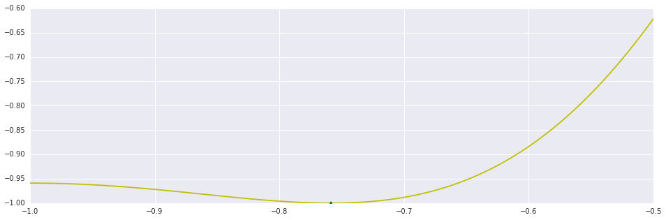
x_dif, n_dif = brent(ftag, (-1.0, -0.5))
x_opt, n_opt = brent_opt(f, (-1.0, -0.9, 0.0), 1e-2, 50)

print "Brent's (derivative): %d Iterations."%n_dif
print "Brent's (objective): %d Iterations."%n_opt

plt.plot(interval_points, f(interval_points), 'y')
plt.plot((x_dif,), (f(x_dif),), 'r*')
plt.plot((x_opt,), (f(x_opt),), 'g.')
plt.show()
Out [10]:
Brent's (derivative): 13 Iterations.
Brent's (objective): 26 Iterations.
(note that there are lots (lots) of possible optimizations, based on annoying bookkeeping, that I haven't included in the implementation above).
6. Differentiable Objectives: A Preview
It's reasonable to expect that differentials would provide useful information for smooth objectives, and that specialized optimization algorithms could utilize it. This is mostly right, which also makes it somewhat wrong. The next post will deal with some of the subtleties, and will overview some specialized algorithms for univariate smooth optimization.
Roughly-speaking, there are two general approaches for those cases: the first is to design bracketing algorithms capable of utilizing derivatives, and the second is to exploit analyticity for deriving a completely different approach for root- finding and optimization (namely, Newton's method, which is the "one notable exception" mentioned earlier).
Both approaches can be generalized to work with multivariate objectives, but variations of Newton's method (a.k.a Quasi-Newton methods) are undoubtedly more common.