Take the Rough With the Smooth

The starting point of the previous post was optimization of differentiable functions, but trying to utilize Fermat's theorem led us eventually to bracketing algorithms, which make no use of the derivative and are applicable for non-differentiable functions.

That's good, but not as good as it sounds. Firstly, non-smooth optimization is very nice - but often the objective of interest is known to be smooth. Reasonably then, taking it into account should improve convergence rate. Secondly, those bracketing algorithms work on univariate objectives. In practice, objectives are usually multivariate - and while adapting bracketing to the multivariate setting is possible, gradient and sub-gradient based methods are often superior in this respect.

This post explores strategies for incorporating derivatives in optimization algorithms, in hope it would lead to improved algorithms. The objective functions are still assumed to be univariate, but it does not render those method pointless. The transition to multivariate objective functions (starting in the next post) will leverage ideas and reuse algorithms from those two posts about univariate functions.

Let's begin with lowering expectation.

Sure, computationally, computing $f$ and $\nabla f$ is equally hard; and yes, theoretically it is indeed possible to accelerate convergence using derivatives. But while it is indeed reasonable to think that an explicit exploitation of smoothness would increase convergence rate, things are actually trickier than that.

Firstly, as we've seen before, in strategies that rely on Fermat's theorem computing just $\nabla f$ is not enough for distinguishing minima from maxima; and a computation of both $f$ and $\nabla f$ pretty much amounts to doubling the computation effort at each step.

Without somehow overcoming this issue, by either efficient approximations or some cleverly reused computations, or by giving up on using Fermat's theorem (for example, as the gradient decent method - to be discussed in an upcoming post - does) using gradients and Hessians is not such a great idea after all.

Secondly, optimization algorithms that do use derivatives are often sensitive to their precision. Obviously, getting the wrong signs of the gradient due to numerical errors does not help anyone's mood, but even less blunt approximation and truncation errors may lead the optimization process astray. For example, the gradient decent method I was just mentioning takes the gradient as the direction of the maximal decent of the objective, which means that in naive implementations even a slightly inaccurate gradients may lead the algorithm to a completely wrong direction.

The same issue may show up in different forms. Notably when using polynomial approximations for the objective. Such ideas are to large extent the basis for second-order line-search algorithms (e.g. quasi-Newton methods), and even more-so with regard to trust-region methods (again, future posts will cover both).

As an demonstration for the potential problem, consider the idea of optimization via polynomial interpolation, e.g. by fitting a polynomial using some high-order derivatives of the objective, and use its optima as an approximation for the target optima. There are actually efficient schemes for doing so by reusing calculated values and minimize function evaluations, so all-in-all the strategy seems plausible.

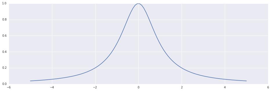
Yet, polynomials are numerically wild. They are wiggly, and their general shape tends to be ill-conditioned with respect to their coefficients. For example (admittedly, a toyetic one), if locally, near an approximated maximum, the objecive looks like this:

Then fitting a polynomial, could look like this:

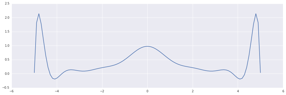
This could be very harmful: most of the effort in solving an optimization problem is invested in getting "close enough" to the optimum. The potential cost of getting thrown away far from the solution may be much higher than the benefits of a possible slightly improved convergence rate.

Dispite the warnings above, there is a useful way to use derivatives in bracketing algorithms. The trick is to to ignore their values, and use only their signs. This makes the algorithm robust under badly approximated gradients, and computationally efficient, since the gradient can be computed only very roughly.

As a matter of fact, this "trick" is common enough in the context of numerical optimization to deserve a promotion to a "technique" (especially in the context of stochastic gradient descent, but that's a whole nother story, to be told in due time).

Let's use this trick in conjunction with the latest bracketing method from the last post, namely Brent's method. This is essentially the same algorithm, but now the sign of the first derivative is used the decide which of the two triplet's sub-intervals is likely to contain the minimum.

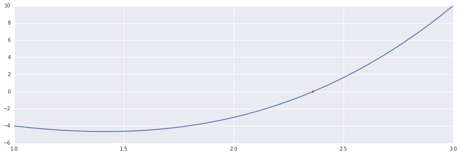
The arbitrary running example in this post will be the function $f(x)=x^3-6x+1$ in the interval $[1, 3]$:

And here's Modified Brent's method in action:

Say you're given a differentiable function $F$ whose roots you'd like to find. Also, say you're name is Newton. So using Taylor series, you obtain $F(x+\delta) = F(x) + J(x)\delta + O(\delta^2)$, and note that if you choose $\delta_0$ such that $J(x)\delta_0 = -F(x)$, then you get $F(x+\delta_0) = O(\delta_0^2)$.

This suggests the iterative scheme $x_{n+1} = x_n + \Delta_n$ where $\Delta_n$ is the solution to the linear system $J(x_n)\Delta_n = -F(x_n)$, which can be reasonably expected to converge to a point $x_0$ such that $F(x_0)=0$ (and it provably does, with some standard fine prints regarding regularity and the goodness of the initial point).

This is Newton's root-finding method:

I think that Newton's method sheds light on the point that opened the previous post: as a root-finding method, Newton's method is effective mainly because it's actually an optimization algorithm in heart, that alternates maximization and minimization steps (i.g. finding roots of $F$ is the same as minimizing $||F||$).

The algorithm that was just presented may find a point outside of the given interval. This is a manifestation of a general problem with the algorithm: there's not guarantee that the iterations monotonically bring us closer to a root (i.e. it's not a "descent method").

A way to mitigate the issue is by combining Newton's method with bracketing: as usual, the algorithm maintains a bracket $(a, b)$ such that $f(a)$ and $f(b)$ have opposite signs, and at each iteration updates one of the endpoints using a Newton step. If it so happens and the step takes the algorithm outside of the current interval, the algorithm reverts to the bisection method. This combination (which comes in several variations) is usually referred to as "Hybrid Newton Method":

You might have noted that the entire discussion about the Newton's method and the Hybrid Newton Method has framed the methods as root-finding algorithms, and not as optimization algorithms. Of course, one of the central points of the current and the previous post was to relate the two concepts. But I opted to deffer the adaptation of those methods for optimization to the next post.

That's because as the notation I've used above may already hinted, unlike all the methods discussed so far, Newton's method can be readily used for multivariate functions $F:R^n\rightarrow R^m$ and be made into a multivariate optimization algorithm. But using this method as-is for this purpose is impractical (due to both numerical and computational reasons). Fortunately, there are effective and practical modifications of it.

The next post will start exploring this landscape.