3. Quasilinearity

As we've seen, computing the DFT by blindly following the definition leads to a quadratic-time algorithm. Now let's see how can it be done asymptotically faster.

Algorithms that compute the DFT of a sequence of length $N$ in $O(N\log N)$ steps are known as Fast Fourier Transforms (FFTs, in short). There are many widely used and excellent implementations of FFTs, such as FFTW, KissFFT and cuFFT.

Their existence is very much NOT a good reason to skip over the algorithmic ideas and implementation details involved: not only it's a bad habit in general (especially when it concerns what is likely "my favorite ever" algorithm), but mostly because it's beneficial: since we're using the DFT exclusively for applications of the convolution theorem, we can actually do better than a general purpose FFT implementation.

The most useful and widely known such algorithms are the Cooley- Tukey family of FFTs. Those algorithms impose some requirements on the length $N$ of the sequences they can transform. Different variations of Cooley-Tukey impose different requirements on $N$, but all of them work only for composite $N$s (a bit of an understatement, "far from prime" would be more accurate). Later we'll see how to leverage a Cooley-Tukey algorithm for the purpose of transforming sequences of arbitrary length.

As for terminology, many specific variations of Cooley-Tukey have their own names (Stockham algorithm and Pease algorithm are two well-known examples). I will discuss those variations in due time, but for the meanwhile I'll consider Cooley-Tukey as a general algorithmic framework for FFT algorithms, and treat uniformly all of its variations.

The efficiency of a Cooley-Tukey implementation is very sensitive to the characteristics of the machine's memory hierarchy and concurrency abilities. In the next few sections those matters will be thoroughly explored.

All Cooley-Tukey algorithms are structured as "divide and conquer" algorithms: at each step they assume that $N$ is a composite-number, $N=N_1N_2$, and decompose the computation into $N_1$ DFTs, each of size $N_2$ (or vice-versa), that can be efficiently combined into a solution of the original problem (actually, by another DFT). In essence, they achieve an asymptotic improvement by exploiting symmetries introduces into the transform by the group-structure of the roots of unity.

The idea goes as following: if $\omega_N=e^{-\frac{2i\pi}{N}}$ is a primitive $N$-th root of unity, then the DFT of $a\in C^N$ (where $N=N_1N_2$) is by definition $\hat{a}_k:=\sum_{n=0}^{N-1}a_n\omega_N^{kn}=\sum_{n=0}^{N_1N_2-1}a_n \omega_{N_1N_2}^{kn}$. This 1-dimensional DFT can be restructured in 2 dimensions (just like array layouts can represent matrices) by the reindexing $k=k_2N_1+k_1$ and $n=n_2+n_1N_2$, that gives: $$\hat{a}_{k_2N_1+k_1}:=\sum_{n_2=0}^{N_2-1}\sum_{n_1=0}^{N_1-1}a_{n_2+n_1N_2}\omega_{N_1N_2}^{(k_2N_1+k_1)(n_2+n_1N_2)}$$

That's where the group structure of the roots of unity comes into play: $$(\omega_{N_1N_2}^{kn})_{n=0,...,N_1N_2-1} = (\omega_{N_1N_2}^{k_2n_2N_1}\omega_{N_1N_2}^{k_1n_2}\omega_{N_1N_2}^{k_2N_1n_1N_2}\omega_{N_1N_2}^{k_1n_1N_2})_{n=0,...,N_1N_2-1} = (\omega_{N_2}^{k_2n_2}\omega_{N_1N_2}^{k_1n_2}\omega_{N_1}^{k_1n_1})_{n=0,...,N_1N_2-1}$$

where the last equality comes from the cancellation property $\omega_{dN}^{dk}=\omega_{N}^{k}$ and the cyclic structure. We conclude: $$\hat{a}_{k_2N_1+k_1}=\sum_{n_2=0}^{N_2-1}[(\sum_{n_1=0}^{N_1-1}a_{n_2+n_1N_2}\omega_{N_1}^{k_1n_1})\omega_N^{k_1n_2}]\omega_{N_2}^{k_2n_2}$$

By switching to the notation $\mathcal{F}_N(\{a_i\}_{i\lt N})_k:=\sum_{n=0}^{N-1}a_n\omega_N^{kn}$, the above result becomes: $$\mathcal{F}_N(\{a_i\}_{i\lt N})_{k_2N_1+k_1}=\sum_{n_2=0}^{N_2-1}[\mathcal{F}_{N_1}(A_{\downarrow n_2})_{k_1}\omega_N^{k_1n_2}]\omega_{N_2}^{k_2n_2}=\sum_{n_2=0}^{N_2-1}[\mathcal{F}_{N_1}(A_{\downarrow n_2})\cdot\vec{\omega}_N^{n_2}]_{k_1}\omega_{N_2}^{k_2n_2}$$

where the symbol $A_{\downarrow n}$ denotes the $n$-th columns in the $N_1\times N_2$ matrix obtained by reindexing $a$ as described above, $\vec{\omega}_N^{n_2}\in C^{N_1}$ has as its $k$-th element the twiddle power $\omega_N^{kn_2}$, and the dot represents point-wise multiplication. Finally, note that the result can rewritten in terms of composite Fourier transforms: $$\mathcal{F}_N(\{a_i\}_{i\lt N})_{k_2N_1+k_1}=\mathcal{F}_{N_2}(\{\mathcal{F}_{N_1}(A_{\downarrow t})_{k_1}\cdot\omega_N^{k_1 t}\}_{t\le N_2})_{k_2}$$

This recursive formulation for the DFT is exactly what we were looking for. Assuming a factorization using $N_2$ is applicable recursively, then its time- complexity $T(N)$ includes $N_2$ recursive applications of $\mathcal{F}_{N_1}$ following by point-wise multiplication of length-$N_1$ vectors, and then $N_1$ recursive applications of $\mathcal{F}_{N_2}$. Thus we obtain the recurrence relation: $$T(N)=N_2T(\frac{N}{N_2})+N_1T(\frac{N}{N_1})+N$$

Since $T(\frac{N}{N_1})=T(N_2)$ is constant, this implies, via the master theorem, a time-complexity of $\Theta(N\log_2{N})$. A more detailed and practical analysis that takes memory hierarchies and distributed decompositions into account will be given later on.

The numerical accuracy of Cooley-Tukey is exceptionally good, since due to its structure, the coefficients it computes are essentially a result of a cascade summation. This is true only if the twiddle factors are computed very precisely, so implementations may use a precomputed tables of accurate twiddle factors. This can be a problem though: for example, GPUs are not really good when it comes to double precision, so it's common to compute the twiddle factors in the CPU and loading the results to the constant memory. But when $N$ gets large (e.g. larger than the constant memory's cache), it can hurt the performance.

The Good–Thomas FFT is similar to Cooley-Tukey, but it's based on a different indexing scheme. In the spirit of the above splitting formula, let $N=N_1N_2$. Then the CRT coordinates $(n_1,n_2)$ of an index $n\lt N$ are the unique simultaneous solutions to $n=n_1\bmod N_1$ and to $n=n_2\bmod N_2$ (and it satisfies $n_1N_2^{-1}N_2+n_2N_1^{-1}N_1$, where the inverse are from the multiplicative groups) and the Ruritanian coordinates $(k_1,k_2)$ of an index $k\lt N$ are the unique solutions to $n_1N_2+n_2N_1=n\bmod(N)$.

The CRT coordinates are well-defined since by the Chinese remainder theorem, any sequence $n_1, ..., n_k$ of $k$ pairwise coprimes positive numbers can be used to uniquely factorize the divisors set of $N=\prod_{i\lt k}{n_i}$. The Ruritanian coordinates are well-defined since the modular equation $n_1N_2+n_2N_1=n\bmod(N)$ has a unique solution, whose components are the unique solutions for $n_2N_1=n\bmod{N_2}$ and $n_1N_2=n\bmod{N_1}$ (both have unique solutions since $\gcd(N_1,N_2)=1$).

From this the Good–Thomas FFT is obtained (here, the output is indexed via CRT coordinates and the input via Ruritanian coordinates): $$\hat{a}_{k_1N_2^{-1}N_2+k_2N_1^{-1}N_1}=\sum_{n_1=0}^{N_1-1}(\sum_{n_2=0}^{N_2-1}a_{n_1N_2+n_2N_21}\omega_{N_2}^{k_2n_2})\omega_{N_1}^{k_1n_1}$$

Note that the formula is very similar to Cooley-Tukey, but without the intermediate multiplications of the terms $\omega_N^{k_1n_2}$ (called twiddle factors), which may give it an advantage in some situations (but not necessarily, because memory access patterns have a huge impact).

Bluestein's algorithm is another FFT that can work on arbitrary $N$s, including prime numbers. It is usually implemented on-top of a variation of a Cooley-Tukey algorithm, and when the structure of $N$ fits the requirement of Cooley-Tukey - it will almost certainly work faster.

The central idea behind Bluestein's algorithm, is to write the DFT $\mathcal{F}(a)$ of a sequence $a\in C^N$ as the convolution $\mathcal{F}(a)_k:=\beta_k^\ast\cdot(\alpha\ast\beta)$ where $\beta_k=e^{\frac{k^2i\pi}{N}}$ and $\alpha_k=a_k\beta_k^\ast$ (and $\ast$, as usual, the is complex conjugation). This comes from just some algebraic manipulations.

Interestingly for us, Bluestein's algorithm works by reformulating the DFT in terms of a convolution that can be computed via another DFT whose structure allow computing via Cooley-Tukey. So in order to compute a convolution $a\ast b$ via Bluestein, we first compute two auxiliary convolutions for computing $\mathcal{F}(a)$ and $\mathcal{F}(b)$, and then a third auxiliary convolution for computing $\mathcal{F}^{-1}(\mathcal{F}(a)\cdot\mathcal{F}(b))$.

The value this reformulation brings, is that the convolution can be computed by padding the sequences with zeros to any desirable length $N'\gt 2N+1$, and then truncating the results of a Cooley-Tukey variant that is optimized for length $N'$. For example, say we have an optimized FFT for $N=2^n$:

Then we can now use Bluestein's to compute the DFT of sequences with arbitrary lengths:

The numerical accuracy of Bluestein's algorithm is an issue for large $N$s, especially when the values $\frac{k^2}{2N}$ are so large that their floating point representation contains little information regarding their fractional part. The reason is that the $\beta_k$s are essentially dependent only on the fractional part of those terms: the function $e^{2zi\pi}$ is periodic and equals to 1 for integer $z$s, thus $\beta_k=e^{\frac{k^2i\pi}{N}}=e^{2i\pi(\frac{k^2}{2 N}-\lfloor\frac{k^2}{2N}\rfloor)}$.

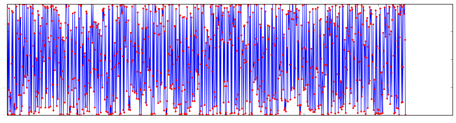
The cause of the problem is a strong hint towards its solution: subtracting large integers from the term $\frac{k^2}{2N}$ when calculating $\beta_k$ keeps the result but eliminates the numerical hazard: $\beta_k=e^{2i\pi\frac{k^2}{2N}}=e^{2i\pi\frac{k^2\text{mod}(2N)}{2N}}$:

To compute $k^2\text{mod}(2N)$ without overflows using $p$-bits integers, write $k^2=k_\text{hi}2^p+k_\text{lo}$ and compute $k^2\text{mod}(2N)=k_\text{hi}[2^p\text{mod}(2N)]+k_\text{lo}\text{mod}(2N)$. Note that $2^p\text{mod}(2N)$ can be precomputed and that for large $N$s it's likely that $k_\text{lo}\lt 2N$, so $k_\text{lo}\text{mod}(2N)=k_\text{lo}$.

Most processors can primitively compute the values of $k_\text{hi}$ and $k_\text{lo}$, so no special code is needed. For example, x86's mull instruction puts them in EDX:EAX and also provides the VPMULHUW instruction in the AVX extension, and CUDA provides the umulhi and umullo instructions.

If $N$ is a prime number, then the indices $\{1,2,...,N-1\}$ can be identified with the cyclic multiplicative group $(\mathbb{Z}/N\mathbb{Z})^\ast$. Denoting its generator by $\mathcal{g}$, it gives two indexing schemes in $\{0,1,...,N-2\}$ by identifying $n$ with its number-theoretically index: $(n\leftrightarrow q)\Leftrightarrow(n=\mathcal{g}^q\bmod{N})$ and $(n\leftrightarrow p)\Leftrightarrow(n=\mathcal{g}^{-p}\bmod{N})$. Thus for $n\ge 1$ we can write $\hat{a}_n=\hat{a}_{\mathcal{g}^{-p}}=a_0+\sum_{q=0}^{N-2} a_{\mathcal{g}^q}\omega_{N}^{\mathcal{g}^{q-p}}=a_0+\alpha\ast\beta^p$ where $\alpha_q=a_{\mathcal{g}^q}$ and $\beta^p_q=\omega_{N}^{\mathcal{g}^{-q}}$ (and $\hat{a}_0=\sum_{k=0}^{N-1}a_{k}$). This is Radar's algorithm.

The convolution in the formula is of two sequences of length $N-1$, and can be recursively computed efficiently, because $N-1$ is a composite number. Moreover, the convolution can be computed by conveniently padding the sequences so their length would match the requirements of an optimized Cooley-Tukey implementation.

The biggest issue with Radar's algorithm is probably the calculation of $\mathcal{g}$, which requires by definition a calculation of a discrete logarithm. This is considered to be practically impossible in general. Luckily, the general problem is of little interest in this context, where $N$ is small. Nevertheless, Radar's algorithm is usually used only to implement hard-coded codelets for small prime numbers, which are later used in the base case of the recursive structure of other FFT algorithms.

The idea behind Radar's algorithm can be generalized to work for powers of primes, i.e., where $N=p^k$ for some prime $p$. The resulting algorithm is called Winograd FFT, and it's usually ineffective on most common architectures.

The base cases for the recursion are hard-coded FFT implementations for small specific $N$s ("codelets"). They should be as efficient as possible, exploiting specific hacks that are particular for their length and numerically accurate (see, for example, Self-Sorting In-Place Fast Fourier Transforms, by Clive Temperton):

Whether larger codelets are required or not depends both on the application and the hardware. If they are needed, they can be devised based on an hard-coded Good–Thomas algorithm (provided the corresponding length is a product of two primes), hard-coded Bluestein or Rader algorithms for prime $N$s, or a carefully direct $O(N^2)$ DFT known as Singleton’s method.

Like the straightforward DFT algorithm, the complexity of Singleton’s method is also $O(N^2)$. But it improves on the straightforward algorithm by a hefty constant factor (0.25 multiplications involved), which makes it attractive as the basis for small-$N$ codelets. Essentially, it does that by exploiting symmetries that allow for the replacement of complex-multiplications with real-multiplications.

Given a sequence $(a_0, a_1,..., a_{N_1})\in C^N$, by definition $\hat{a}_k=a_0+\sum_{n=1}^{\frac{N-1}{2}}a_ne^{-\frac{2\pi ikn}{N}}+\sum_{n=1}^{\frac{N-1}{2}}a_{(N-n)}e^{-\frac{2\pi ik{(N-n)}}{N}}$. Since $\cos(\frac{2\pi(N-n)k}{N})=\cos(\frac{2\pi nk}{N})$ and $\sin(\frac{2\pi(N-n)k}{N})=-\sin(\frac{2\pi nk}{N})$, by calculating -

• $A_k^+:=\mathrm{Re}(a_0)+\sum_{n=1}^{\frac{N-1}{2}}{(\mathrm{Re}(a_n)+\mathrm{Re}(a_{N-n}))\cos(\frac{2\pi nk}{N})}$
• $A_k^-:=-\sum_{n=1}^{\frac{N-1}{2}}{(\mathrm{Im}(a_n)-\mathrm{Im}(a_{N-n}))\sin(\frac{2\pi nk}{N})}$
• $B_k^+:=\mathrm{Im}(a_0)+\sum_{n=1}^{\frac{N-1}{2}}{(\mathrm{Im}(a_n)+\mathrm{Im}(a_{N-n}))\cos(\frac{2\pi nk}{N})}$
• $B_k^-:=-\sum_{n=1}^{\frac{N-1}{2}}{(\mathrm{Re}(a_n)-\mathrm{Re}(a_{N-n}))\sin(\frac{2\pi nk}{N})}$

we obtain $\hat{a}_k=(A_k^+-A_k^-)+i(B_k^++B_k^-)$ for $k\le\frac{N-1}{2}$ and $\hat{a}_{N-k}=(A_k^++A_k^-)+i(B_k^+-B_k^-)$ for $k\gt\frac{N-1}{2}$. For further details, see Gough.

For convolutional networks, in which the length of the filters are very loosely constrained, the only real factor is the hardware. For GPUs the codelets above are typically more than enough, but for CPUs it might be worth to invest in a larger family of codelets.

The Cooley-Tukey formula $\mathcal{F}_N(\{a_i\}_{i\lt N})_{k_2N_1+k_1}=\mathcal{F}_{N_2}(\{\mathcal{F}_{N_1}(A_{\downarrow t})_{k_1}\cdot\omega_N^{k_1 t}\}_{t\le N_2})_{k_2}$ for $N=N_1N_2$ can be translated to an algorithm by, for example, following those steps:

1. Reshape the sequence as a matrix.
2. Transform the columns of the reshaped sequence.
3. Transpose the transformed matrix.
4. TMultiply the columns of the transposed matrix by the appropriate factors (known as Twiddle Factors).
5. Transform again the columns of the final matrix.

Here's a pythonic prototypes for those steps:

I acknowledge that emphasizing the transposition as a separate step may seem silly at first, especially when looking at the Python code in which it's utterly trivial. But this triviality is misleading, and it will soon become clear that many core-issues with implementing FFTs can be reduced to difficulties with this step.

At this point, the reason that Cooley-Tukey algorithms are restricted only to special values of $N$ should be clear: their recursive structure relies on $N$'s factorization. The simplest constrains an implementation can impose over the length $N$, is the requirement $N=r^n$, where $r$ is a natural number called the radix. The smallest and atomic FFTs used in the base-cases of the recursion, are commonly known as butterflies, due to the way they appear in data-flow diagrams of the algorithm. The most widely-known (though not most-widely useful) FFT is probably the fixed-radix $r=2$ Cooley-Tukey algorithm.

There are many other variations, with important implications for the performance profile of the implementation. For example, mixed-radix FFTs assume that $N$ has a small number of small factors, such as $N=2^a3^b$, and split-radix FFTs also assume $N=r^n$, but then alternate the radix, e.g, they may assume $N=2^n$ and use the radixes 2 and 4. Another common variation relates the radix to $N$, for example by choosing $r=\sqrt{N}$. The trade-offs involved in imposing different requirements on the factorization of the length $N$ are effected mostly by the structure of the memory hierarchy. More on this soon.

Any of those variations can be implemented rather simply by reusing the above methods as building blocks. For starters, consider fixed-radix algorithms. Their implementation require one to choose whether to keep $N_1$ fixed as $N_1=r$ and constantly set $N_2=\frac{N}{r}$ - which is said to be decimation in time, or on the contrary, to fix $N_2=r$ and constantly set $N_1=\frac{N}{r}$, which is called decimation in frequency:

The two variations look very similar, but they differ in some significant aspects. Most notably, the structure of the decimation in frequency variation is naturally tail-recursive, while the structure pf the decimation in time variation is not, and the two exhibit different memory access patterns. This issue is central to efficient application of the Fourier transform for convolutions.

Due to the non-tail-recursive character of DIT, the straightforward way of understanding it is as a divide and conquer algorithm, or as the trendy cool kids call it nowadays, map- reduce (yes, I'm well aware of the technical difference, but more interested in the structural similarities).

Here's a schematic example of how a radix-3 decimation in time algorithm operates on a sequence of length $3^4$:

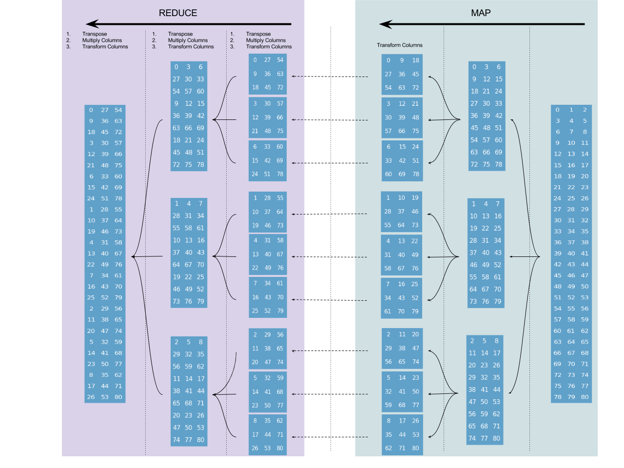
Each node (blue rectangle) represents a stack-frame, and the numbers in it are used as a notional tool to align the layouts of the nodes with the layouts of their parents. In the case of DIT those numbers are the indices of the sequence on which it operates (assuming an in-place operation), and can be thought of as relative memory address. So the diagram offers a visualization for the memory access patterns of the algorithm.

In the "map" phase the algorithm does nothing than divisions of the input, until square-matrices (whose dimension is determined by the radix $r$) are obtained - whose columns are then transformed (using a base-case Fourier transform for length $r$ sequences). In each frame in the "reduce" step, the corresponding matrix is transposed, its columns are multiplied by the twiddle factors and then transform using again the base-case Fourier transform for length $r$ sequences (the matrices columns are always of length 3, all the way up).

For comparison, here's a similar diagram for radix-3 decimation in frequency algorithm (also with an input sequence of length $3^4$):

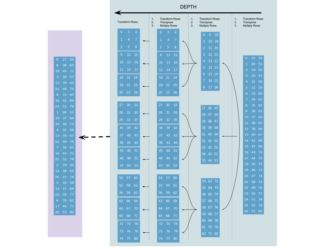
Since decimation in frequency is tail-recursive (the forth and last step is the base-case transform), it has a simple recursive structure, without fancy reductions. Again, the numbers in the nodes are used for aligning the layouts of the nodes with their parents. But unlike the previous case, they are no longer indexing the sequence itself. Here they are "relative address" (with respect to the node parent), and not absolute addresses. The final absolute address are shown above over the purplish background.

This is possibly the most important issue at this point. When doing decimation in time, the transpositions "go upward" in the recursion tree, and when doing decimation in frequency, the transpositions "go downward" in the recursion tree.

For a simple radix-2 FFT it's not hard to deduce the way it access memory. Essentially, each step in the radix-2 DIT recursion splits the input sequence into the odd and even sub-sequences, and each step in the radix-2 DIF recursion splits the input sequence into two sequential halves. This basically means that the DIT variation works by processing a scrambled permutation of the spatial- sequence, and ends by processing the spectral sequence in the right order, while the DIF variation starts by processing the spatial-sequence in the right order, and ends by processing a scrambled permutation of the spectral sequence. This is generally true, and will be explored later.

Before going deeper into the exploration of the "FFT landscape", it would be beneficial to reformulate algebraically the splitting lemma by using matrix notation. This simplifies things greatly, both by allowing the production of new algorithmic variations by applying formal transformations and by emphasizing the memory access patterns and modular decompositions of the different variations.

The algebraization the formula $\mathcal{F}_N(\{a_i\}_{i\lt N})_{k_2N_1+k_1}=\mathcal{F}_{N_2}(\{\mathcal{F}_{N_1}(A_{\downarrow t})_{k_1}\cdot\omega_N^{k_1 t}\}_{t\le N_2})_{k_2}$ is - $$\mathcal{F}_{N}=(\mathcal{F}_{N_2}\otimes I_{N_1})W_{N_2}^{N_1}T_{N_1}^{N_2}(\mathcal{F}_{N_1}\otimes I_{N_2})$$

where -

1. $\mathcal{F}_n$ is the $n\times n$ DFT matrix.
2. $I_n$ is the $n\times n$ identity matrix.
3. $W_{n}^{m}$ is diagonal $nm\times nm$ matrix of twiddle factors satisfying $W_{n}^{m}[i,i]=\omega_{nm}^{sr}$ where $i=sm+r$.
4. $T_{n}^{m}$ is a $nm\times nm$ permutation matrix such that $T[i,j]=1$ if $i=rn+s$ and $j=sm+r$ (and $T[i,j]=0$ otherwise).
5. The operation $\otimes$ is the Kronecker Product.

It's nicely interpretable: Firstly, note that the permutation $T_{n}^{m}$ operates on a vector $x\in C^{nm}$ by transposing the $n\times m$ matrix whose row-major sequential representation is given by $x$. And secondly, note that if $A_n$ is a $n\times n$ matrix, then the matrix $A_n\otimes I_m$ operates on a vector $x\in C^{nm}$ by reshaping it as a row-major $n\times m$ matrix and transforming its $m$ columns (each of length $n$) by $A_n$. Similarly, $I_m\otimes A_n$ operates on a vector $x\in C^{nm}$ by reshaping it as a row- major $m\times n$ matrix and transforming its $m$ rows (each of length $n$) by $A_n$.

Now by using purely algebraic manipulations, such as $(A\otimes B)(C\otimes D)=AC\otimes BD$, $(A\otimes B)^T=A^T\otimes B^T$ and $I_{mn}=I_m\otimes I_n$, new algorithmic variations can be simply derived. For example, it's clear that any splitting has a dual form given by its formal transposition, which is a generalization of the DIT/DIF duality that was previously introduced for fixed- radix algorithms.

It's instructional to also see that constructively defined:

The memory access pattern of an implementation for a Cooley–Tukey algorithm is a key-factor in its performance. Algebraically, the memory access pattern is controlled by the Kronecker products and the permutation matrix in the specific splitting on which the implementation is built.

Let's consider an iterative implementation of a Cooley–Tukey algorithm. Starting with a factorization of the sequence length $N=\prod_{i\le n}N_i$ (the vector $(N_0, N_1, ..., N_n)$ is called the radix vector), and recursively expending the formulation above $\mathcal{F}_{N}=(\mathcal{F}_{N_2}\otimes I_{N_1})W_{N_2}^{N_1}T_{N_1}^{N_2}(\mathcal{F}_{N_1}\otimes I_{N_2})$, the following formula emerges: $\mathcal{F}_{N}=\prod_{i\le n}(T_{q_i}^{N_i}W_{q_i}^{N_i}\otimes I_{p_{i-1}})(\mathcal{F}_{N_i}\otimes I_{m_i})$ where $p_i=\prod_{k\le i}N_k$, and $q_i=\frac{N}{p_i}$, and $m_i=\frac{N}{N_i}$. This is a decimation in frequency algorithm, and its formal transposition gives a decimation in time algorithm.

This iterative algorithm, like the recursive algorithm given before, requires performing a sequence of transpositions. One way to deal with it, is the obvious way: by just performing a sequence of actual transpositions. The problem is that on modern computers a transposition of large matrices is anything but simple.

Consider an implementation for an out-of-place transposition of $N_1\times N_2$ matrix. The simplest and most naive implementation would be to use a pair of nested loops. Well, even this simplest of simple methods is hard to manage. Consider the following implementation, meant to be executed on a CPU:

How this code exactly behaves obviously depends on the specifics of the CPU and the values of $N_1$ and $N_2$. And while the general problems it has with respect to cache locality are obvious, the fact that those problems are asymmetric in $N_1$ and $N_2$ is not, and so is the fact that it performs worse when $N_1$ (or $N_2$) is a power of two. From a cache-locality point of view, the cases $N_1\gt N_2$ and $N_1\lt N_2$ seem equally bad, yet $N_1\gt N_2$ is faster (for square matrices, the column-major algorithm is faster).

This rabbit hole goes rather deep. Measurements made it clear that it has nothing to do with some asymmetry between reads and writes in the CPU's pre- fetching mechanism, as I first suspected. Instead, apparently it's mainly because that in order to guarantee a relaxed memory consistency model, a CPU with an out-of-order pipeline must perform memory disambiguation for all the in-flight stores in order to eliminate the possibility of a memory dependencies violation. So having many loads and few stores in-flight, is much better than having few loads and many stores in flight. If the cache implements a write-allocate policy, it might also have a (smaller) effects in the same direction.

The problem with powers-of-2, on the other hand, is the occurrences of more cache-line conflicts than the cache's set associativity can mitigate. And if we were to parallelize this method on a multi-core machine, we would have to consider the specific coherence protocols of the target platform. Let's walk away very slowly from this line of thought.

In order to make a remotely efficient transposition, the above algorithm must be re-factored into a procedure that exhibit spatial locality. The usual approach is to work in small blocks, that each can be transposed "in-cache". Assuming the block size divides both $N_1$ and $N_2$, this is the algorithm:

A major drawback of this method, is that it's sensitive to the specific details of the memory hierarchy (which determines the optimal block size). But applying the same reasoning recursively leads to an (almost) cache-oblivious algorithm:

This is just "almost" cache-oblivious, since specifics such as the order of an associative cache may still play a factor in the overall performance of the algorithm. A very similar approach is used in the parallelization of the transposition algorithm. In this context the blocks are known as "tiles", and the role of "annoying specificalities" fulfilled by cache-associativity, goes to shared-memory bank conflicts.

A very important issue with explicit transpositions, is that an efficient in- place transposition of non-square matrices is a nightmare. So usually, such implementations simply don't work in-place and require extra storage. Sometimes it's an acute problem, and sometimes not so much. For example, in some parallelized implementations the "matrix transposition" step can be often assimilated with the communication mechanism used for parallelization. In pseudo-code it'd look roughly like this:

In OpenCL the relevant API is mainly async_work_group_strided_copy.

Instead of performing a sequence of transpositions, the algebraic formulation of the algorithm can be modified so that all the permutations are performed once. This key observation is the identity -

which implies - $$\begin{multline} \mathcal{F}_{N}=(\mathcal{F}_{N_2}\otimes I_{N_1})W_{N_2}^{N_1}T_{N_1}^{N_2}(\mathcal{F}_{N_1}\otimes I_{N_2})\\ =(\mathcal{F}_{N_2}\otimes I_{N_1})W_{N_2}^{N_1}T_{N_1}^{N_2}T_{N_2}^{N_1}(I_{N_2}\otimes\mathcal{F}_{N_1})T_{N_1}^{N_2}\\ =(\mathcal{F}_{N_2}\otimes I_{N_1})W_{N_2}^{N_1}(I_{N_2}\otimes\mathcal{F}_{N_1})T_{N_1}^{N_2} \end{multline}$$

In order to derive a useful recursive relation, note that for any arbitrary $m,k\in N$ the following recursion holds: $$(I_m\otimes\mathcal{F}_{N}\otimes I_k) = (I_m\otimes\mathcal{F}_{N_2}\otimes I_{N_1k})(I_m\otimes W_{N_2}^{N_1}\otimes I_k)(I_{N_2m}\otimes\mathcal{F}_{N_1}\otimes I_k)(I_m\otimes T_{N_1}^{N_2}\otimes I_k)$$

This motivates the definitions - $$\begin{align} &\mathcal{F}(m, N, k) := I_{m}\otimes\mathcal{F}_{N}\otimes I_{k}\\ &W(m, N_1, N_2, k) := I_m\otimes W_{N_2}^{N_1}\otimes I_k\\ &T(m, N_1, N_2, k) := I_m\otimes T_{N_1}^{N_2}\otimes I_k \end{align}$$ that allows rewriting the recursion more cleanly as: $$\mathcal{F}(m, N_1N_2, k)= \mathcal{F}(m, N_2, N_1k)W(m, N_1, N_2, k)\mathcal{F}(N_2m, N_1, k)T(m, N_1, N_2, k)$$

This recursive relation can be used to construct an iterative algorithm with no intermediate transpositions by following the same processes used to construct the previous iterative algorithm. The resulting DIT algorithm is given by - $$\mathcal{F}_{N_1N_2...N_k}=\prod_{j\ge 1}(I_{N_1...N_{j-1}}\otimes\mathcal{F}_{N_j}\otimes I_{N_{j+1}...N_k})(I_{N_1...N_{j-1}}\otimes W_{N_j}^{N_{j+1}...N_k})\tau$$

where $\tau$ is the product of all permutations, whose structure is revealed by considering Mixed-Radix Positional Systems.

The usual interpretation of a numeral symbol, such as $1729$, is as a positional notation: the position of the $i$-th digit carries the magnitude $10^i$, and so it represents the number $9\cdot10^0+2\cdot10^1+7\cdot10^2+1\cdot10^3$. This is a radix-10 positional notation system, but of course many other positional notation system are common (binary, hexadecimal etc).

But another equally valid interpretation of $1729$ (and numeral symbols in general) is as the coordinates $(9,2,7,1)$ of a spatial position in a 4-dimensional array whose dimensions are $(10, 10, 10, 10)$. This interpretation gives the natural numbers a geometric layout (of a tensor space). It also leads naturally to the concept of mixed-radix positional systems, in which instead of a fixed radix $r$ (such as 2, 10 or 16), there is a (often finite) sequence of radixes $(r_0, r_1, ...)$ - and the position of the $i$-th digit (now switching to little-endianness convention) carries the magnitude $\prod_{s=1}^ir_s$. The vector $(r_0, r_1, ..., r_n)$ is called "the radix-vector", and the representation of a number, its coordinates, is called a "digit vector". The usual fixed-radix positional systems are a special case in which $r_0=r_1=...=r_k=...$

Mixed-radix positional system are very common. For example, any computer program that uses multidimensional arrays works with a mixed-radix positional system, and so are many units of measure ("Four score and seven years ago"...). As an another example, the radix-vector $(1, 2, 3, 4, ...)$ gives the factorial-number system, in which every positive integer can be written uniquely as the sum of the factorials it bounds. This system is used in algorithms for permutation tests see Knuth's TAOCP, volume 2).

Given a finite radix vector $R=(r_0,r_1,...,r_k)$, we denote $Z^R:=[0,r_0]\times[0,r_1]\times...\times[0,r_k]\subset Z^k$, and $|R|:=\prod_ir_i$. A mixed-radix positional system is a bijection $\mu_R:Z^R\leftrightarrow Z^{|R|}$ given by $\mu_R(d)=\sum_{i=0}^{k-1}d_in_0...n_{i-1}$, where a $d\in Z^R$ is digit vector. This works exactly like in the usual fixed-radix positional systems:

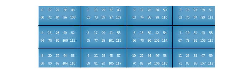
Any permutation $\pi\in S_k$ induces an action $\mu_\pi$ over $Z^{|R|}$ by permuting the digits of its representation in $Z^R$. Such permutations are called Index-Digit Permutations:

The definitions in the recursion above can now be parsed as relations over the elements of a sequence whose length is $mN_1N_2k$, defined in terms of their position when expressed by using the radix vector $(m, N_1, N_2, k)$. Geometrically, it means that the sequence is layout as a nested grid, of $m\times N_1$ cells that each is a $N_2\times k$ matrix.

For example, the layout of a sequence of length $4\cdot3\cdot5\cdot2$ with respect to the radix-vector $(4,3,5,2)$ is of a $4\times 3$ grid whose cells are $5\times2$ matrices. In the following diagram the numbers are indexes, and their location is their mixed-radix representation:

With this image in mind, the action of $T(m, N_1, N_2, k) := I_m\otimes T_{N_1}^{N_2}\otimes I_k$ can be interpreted combinatorially as the index-digit permutation induces by the exchange $(m, N_1, N_2, k)\rightarrow(m, N_2, N_1, k)$, which is just a spatial swap. Now the overall effect of all the permutations performed by a FFT with a given factorization, denoted here as $\tau$, can be derived by induction, based on the observation that index-digit permutations behave nicely with respect to subordination, which means that they can work on "blocks" of digit (e.g. mixing the digits of an hexadecimal number, is like mixing the nibbles of its binary representation). The result is that $\tau$ itself is also an index-digit permutation, with respect to the radix- vector $(N_1, N_2, ..., N_k)$, that is generated by the reversal permutation.

Such a permutation is call Index-Digit Reversal, and performing it on the inputs as a preliminary step, allows applying a DIT transform that does not contain any transpositions. Similarly, it's possible to perform a transposition- free DIF transform following by an index-digit reversal of the outputs:

The main value of digit-reversal permutations, is that they allow an easy implementation of in-place FFT algorithms. But the permutation itself is not trivial to do, and usually don't really lead to any improvement in the algorithm performance (and may even worsen things). That's mainly because it requires unfriendly memory access. I won't get into it here (see, for example, the Gold- Rader or Rodriguez's algorithms) because I'd like to focus on convolutional nets, for which - as I shall soon explain - this strategy is not really useful.

The analysis above , on the other hand, wasn't a waste of time. It is very useful as a guidance for designing efficient algorithms, and the mapping of a number to its digit-reversal dual is a useful building-block. Many algorithms on many platforms are not very sensitive to this step, and a relatively simple function should do. e.g for radix-2 (See here a nice discussion regarding implementation details):

A third strategy for dealing with the permutations (aside from explicitly performing arbitrary transpositions, or pre-sorting), is to use a variation of Cooley-Tukey in which the recursive-decomposition require only transpositions of square-matrices (which can be done in-place). Such algorithms are called self- sorting in-place FFTs (e.g. the Johnson-Burrus algorithm).

The key insight for those algorithms is that, as I showed earlier, $T(m, N_1, N_2, k) := I_m\otimes T_{N_1}^{N_2}\otimes I_k$ is actually a multidimensional transposition, hence can be easily performed in-place whenever $N_1=N_2$. Moreover, for $N_1,N_2,N_3\in Z$ the product $T(m, N_1, N_2N_3, k)T(mN_1, N_3, N_2, k)$ is also a multidimensional transposition, with respect to the radix- vector $(m,N_1,N_2,N_3,k)$ and the exchange $(1,2,3,4,5)\leftrightarrow(1,4,3,2,5)$. Thus any recursive step for a sequence whose length is non-square-free (say, $NR^2$) can be splitted by using a square- transposition, executable in-place: $$\mathcal{F}(m, NR^2, k)=\mathcal{F}(mRN, R, k)W(m, RN, R, k)T(m, R, RN, k)T(mR, N, R, k)\mathcal{F}(mR, N, Rk)W(mR, N, R, k)\mathcal{F}(mRN, R, m)$$

Since this strategy is also not very useful in the context of convolutional networks, I leave it at that. A good source on this subject is Hegland.

An important aspect of the recursive decomposition, is the effect of the sub- problems' sizes on the performance, due to their impact on the locality of reference. This issue has many forms, and the situations that occur in hierarchical memory systems (e.g. SMP with caches), NUMA machines, and heterogeneous systems (e.g. a CPU/GPU machine) are all similar.

Consider a sequence of length $N$ and a fixed radix-$r$ transform. So the entire sequence is transformed by combining many transformations of sequences whose length is $r$. Specifically, there are $\log_rN$ steps, and each step involves $\frac{N}{r}$ transforms. Thus there are $\Theta(\frac{N}{r}\log_rN)$ small transforms.

If each computing-unit has a local-memory of size $r$, then each time it performs a transformation it access $r$ times the global memory. Denoting $Q(N;r)$ the number of references to the global memory (or equivalently, from a message-passing perspective - the number of inter-node messages), a radix-$r$ algorithm satisfies $Q(N;r)=\Theta(r\frac{N}{r}\log_rN)=\Theta(N\log_rN)$.

A previous calculation showed that a fixed-radix Cooley-Tukey algorithm has a time-complexity of $\Theta(N\log_2{N})$. But now it's clear how realistically the execution time may depend on the radix $r$, and it turns out that choosing an arbitrary small radix (e.g. $r=2$) is a bad idea. The radix should be as large as the local memory available for the computing units.

It's often desirable to deign an algorithm that is not optimized to a very specific platform, and is insensitive to the size of the local-memory. Note that this concept of cache-obliviousness is as valid when caches are not an important factor, as when writing code for GPUs (where the local-memory is used very explicitly, regardless of caching which plays a different role in this context).

Probably the most important factor in such cache-obliviousness FFTs, is the traversal plan over the recursion trees: a depth-first traversal pretty naturally leads to cache-obliviousness. While a breath-first radix-2 is actually an "optimal" cache-oblivious FFT in the sense it maximizes access to global memory, a depth-first radix-2 has near-optimal access rate of $\Theta(N\log[\frac{N}{Z}])$ where $Z$ is the size of the local memory (though of course the algorithm itself does not use $Z$ explicitly, as it is a radix-2 algorithm).

The optimal choice is not $r=2$, but $r=\sqrt(N)$, known as the "four-step FFT". The number of accesses to global memory of this algorithm is $\Theta(N\log_ZN)$ (and again, the algorithm itself does not use $Z$ explicitly). In practice, though, more complex schemes are usually used (with better constant factors) - especially in asymmetric heterogeneous or multi-core systems.

Implementations of both DIT and DIF algorithms have a considerable amount of freedom as for the traversal of the recursion tree. They can of course choose to traverse it depth-first (post-order) or breath-first, but they also may choose a mixed traversal strategy (e.g. breath-first up-to some level, and depth-first from there on) or a non-deterministic traversal plans (which may occur naturally in concurrent implementations). Note that all of this applies just the same for mixed-radix and split-radix algorithms. Probably the most important factor in choosing a traversal strategy is the spatial and temporal locality it presents.

Both DIF and DIT algorithms can be implemented, recursively, iteratively and concurrently, and this independent from the choice of traversal strategy. Together with the radixes, we face a pretty large combinatorial space of algorithms and implementations. Libraries such as FFTW invest lots of efforts in exploring this space for choosing a near-optimal variation for a given concrete problem on a specific hardware.

Let's explore those options a bit. The goal would be to have some algorithms that explicitly traverse the recursion trees, and produce the appropriate memory access pattern. The implementations bellow are meant to be as explicit as possible, and are meant to be mainly pedagogically useful, to provide insights and serve as a basis for explorative modeling of algorithmic strategies.

To make their form as uniform as possible, it's useful to have methods that generate the indices matrix associated with the nodes in the recursion tree, as a function of the depth-index and the breath-index:

The whole point of the following code is exploration of the memory access patterns, but it can be easily used to actual implement FFTs, e.g. by using those two useful methods:

Using this formulation, the problem is reduces to general traversal over complete k-ary trees. Breath-first implementations, weather recursive or iterative, are the simplest (the depth is truncated since the FFT algorithms work with matrices in their leafs):

Recall that the DIF traversal is pre-order and the DIT traversal post-order, so, for example:

Depth-first traversal is a somewhat more complicated. Recursive schemes are still simple:

But iterative schemes are messier. Unlike some rumors that go around, for non- concurrent implementations iterative implementations have little to no advantage over recursive onces. They are still important though, mostly because they allow for an explicit task scheduling.

For example, to iteratively traverse depth-first in order, the algorithm jumps from the last leaf in the branch to the parant, in then traverse upwards until it jumps again directly to leaf:

In practice, it could be more reasonable to recurse or iterate directly over the values of stride, rows and offset instead of over the depth and breadth indices - and thus save some computations. The modified indices generating methods are:

The modifications of the recursive traversal methods are straightforward for either DIT or DIF (the stride is increased or decreased by a factor of the radix with the depth, etc), but the iterative methods needs now to mimic more closley the dynamics of a stack.

An implicit iteration of a complete k-ary tree amounts to a sequential generation of UP and DOWN instructions that correspond to the desirable traversal strategy (per-order, in-order and so on). A general purpose implicit iteration scheme can be used to translate very general recursive algorithms to iterative algorithms - often without requiring additional storage space (e.g. a stack, or for memoization).

One way to do it, is by maintaining a counter for the visited leafs $m$ and the current implicit depth $d$. Actually, the depth itself is used indirectly for calculating the count of leafs the subtree rooted in the current implicit node has, which is given by $s:=k^{\log_kN-d+1}$ where $N$ is the total number of nodes. So instead of maintaining the implicit depth, it's preferable to maintain the "subtree size" $s$ directly. Leafs can be easily identified by their implicit depth (or a subtree size of 1).

So each issuing of an UP instruction increases the visited-leafs counter if the current implicit node is a leaf, and always decreases the depth (or equivalently, increases the subtree-size by a factor of $k$), and each issuing of a DOWN instruction increases the depth (or equivalently, decreases the subtree-size by a factor of $k$).

Some additional bookkeeping is needed for maintaining the relative position $i$ of the current implicit node with respect to its implicit siblings. Each UP instruction sets it to $i=\frac{m}{s}\%k$ and each DOWN instruction sets it to $i=\frac{mk}{s}\%k$.

Now, for an implicit post-order DFT traversal, the algorithm issues an UP instruction whenever it encounters a leaf or $m=si$m and a DOWN instruction otherwise.

There's a direct correspondence between the matrix formulation of a FFT algorithm to its parallelization.

Consider the vector $x:=(x_1,...,x_n)\in F^{mk}$ as $m$ vectors of length $k$, denoted $v_i=(x_{ki},x_{ki+1},..,x_{k(i+1)-1})\in F^k$. Similarly, consider $y:=(A_m\otimes I_k)x\in F^{mk}$ as $m$ vectors of length $k$, denoted $w_i=(y_{ki},y_{ki+1},..,y_{k(i+1)-1})\in F^k$. Then $w_j=\sum_{i\le m}\alpha[i,j] v_i$, where $\alpha[i,j]$ are $A_m$'s elements. So $(A_m\otimes I_k)$ can be computed by $m$ vectorized expressions, each works on (the same) $m$ vectors of length $k$.

Now, consider the vector $x:=(x_1,...,x_n)\in F^{mk}$ as $k$ vectors of length $m$, denoted $v_i=(x_{mi},x_{mi+1},..,x_{m(i+1)-1})\in F^m$, and similarly, consider $y:=(I_k\otimes A_m)x\in F^{mk}$ as $k$ vectors of length $m$, denoted $w_i=(y_{mi},y_{mi+1},..,y_{m(i+1)-1})\in F^m$. Then $w_i=A_m v_i$, and $I_k\otimes A_m$ can be computed by $k$ independent transformation, each applied on a different vector.

Thus, the product $I_k\otimes A_m$ represents a distributed algorithm suited for block-parallelism while $A_m\otimes I_k$ represents a vectorized computation suited for vector-parallelism. In that sense, block-parallelism and vector- parallelism are dual to each other.

There are other practical considerations that are algebraically expressible. For example, the length of the vectors in the resulting algorithm (the value of $k$ in the terms $I_k\otimes A_m$) which should be fixed for SIMD architecture, bounded for GPUs or maximal for vector-machines. Another example, relevant for block-parallelism on multi-core machines, is the size of the cache lines: an efficient algorithm should respect to the cache lines boundaries when applying in-block permutations (e.g. permute only elements the share the same cache-lines, or permute entire cache-lines globally - but never exchange two elements from 2 different cache-lines). And a third example, is the usage of digit-reversal permutations which (if required) should be restricted to one compute-unit, and preferably work entirely locally in the present of a memory-hierarchy.

From all of the above, it's clear that a major difficulty with efficient implementations of Quasilinear algorithms for the Fourier-transform comes from problematic memory-access patterns induced by the index-digit permutations involved in recursive formulations of the DFT.

But recall that such algorithms were relevant to begin with because of the convolution-theorem $a\ast b=\mathcal{F}^{-1}(\mathcal{F}(a)\cdot\mathcal{F}(b))$. Also recall that as we saw, decimation in frequency without the said permutations works on an ordered spatial sequence and outputs a digit-reversed spectral sequence, while a decimation in time without those permutations can be seen as working on a digit-reversed spatial sequence, and resulting an ordered spectral sequence.

Since the same holds for the corresponding inverse-transforms, it's possible to design convolution algorithms that can be significantly more efficient than general-purpose transforms.

In details, fix some mixed-radix positional system, and denote by $\mathrm{DIT}_N(a), \mathrm{DIF}_N(a), \mathrm{IDIT}_N(a)$ and $\mathrm{IDIF}_N(a)$ the permutation-free $C^N\mapsto C^N$ transforms, and by $\rho_N$ the digit-reversal permutation. Then for any $a\in C^N$:

As can be simply verified:

Where for this demonstration I've used a naive radix-2 implementation:

So instead of a mindless application of the convolution theorem (multiplications are pointwise) -

things can be simplified to -

Or in code:

Note that the pointwise multiplication here is NOT of the transformed sequences, but of a permuted versions of them. Also note that other variations, such as $a\ast b = \mathrm{IDIF}_N(\mathrm{DIT}_N(a)\mathrm{DIT}_N(b))$ won't work, because the pointwise multiplication is gibberish (it's of transformed permutated sequences, and not of permuted transformed sequences).

Convolutional layers are typically restricted to real numbers. That's another optimization opportunity.

For any real sequence $a\in R^N$, its DFT satisfies $\hat{a}_k=\hat{a}_{N-k}^\ast$ where $\ast$ is the complex conjugate. This means that the computation is half the size of that of an equally long complex sequence (and customized functions can be space-optimized to deal only with real inputs).

For notational simplicity, assume $4|N$. Denote by $\mathcal{RF}_N$ a "real version" of the Fourier transform $\mathrm{F}_N$ that computes only the first $\frac{N}{2}+1$ elements, so $\mathcal{RF}_N:R^{N}\rightarrow C^{\frac{N}{2}+1}$. It satisfies $\mathcal{RF}_N(\{a_{i\lt N}\})_j = \mathcal{F}_N(\{a_{i\lt N}\})_j$ for $0\le j\le\frac{N}{2}$, and by the fundamental symmetry for the reals it also satisfies $\mathcal{RF}_N(\{a_{i\lt N}\})_{N-j}^\ast = \mathcal{F}_N(\{a_{i\lt N}\})_j$ for $\frac{N}{2}\lt j\lt N$.

When $N=N_1N_2$, the Cooley-Tukey splitting is: $$\mathcal{F}_N(\{a_i\}_{i\lt N})_{k_2N_1+k_1}=\mathcal{F}_{N_2}(\{\mathcal{F}_{N_1}(A_{\downarrow t})_{k_1}\cdot\omega_N^{k_1 t}\}_{t\le N_2})_{k_2}$$

for $k=k_2N_1+k_1$ with $0\le k\lt N$ and $0\lt k_1\lt N_1$. Similarly, for $\mathcal{RF}_N$, we can write:

$$\mathcal{RF}_N(\{a_i\}_{i\lt N})_{k_2N_1+k_1}=\mathcal{RF}_{N_2}(\{\mathcal{RF}_{N_1}(A_{\downarrow t})_{k_1}\cdot\omega_N^{k_1 t}\}_{t\le N_2})_{k_2}$$

which again holds for $k=k_2N_1+k_1$, but this time with $0\le k\le \frac{N}{4}$ and $0\lt k_1\lt N_1$.

To complete its definition, use the real symmetry again to obtain:

$$\mathcal{RF}_N(\{a_i\}_{i\lt N})_{k_2N_1+k_1}=\mathcal{RF}_{N_2}(\{[\mathcal{RF}_{N_1}(A_{\downarrow t})_{(N_1-k_1)]^\ast}\cdot\omega_N^{k_1 t}\}_{t\le N_2})_{k_2}$$

for $k=k_2N_1+k_1$ with $\frac{N}{4}\lt k\lt \frac{N}{2}$, and note that $\mathcal{RF}_N(\{a_i\}_{i\lt N})_{\frac{N}{2}} = \sum_{t=0}^{N_2}(-1)^{t}\mathcal{RF}_{N_1}(A_{\downarrow t})_{\frac{N}{4}}$.

In practice, the fact that the $0$th and the $\frac{N}{2}$th elements are real can be used to gain some additional minor optimization.

In code (for recursive decimation in time, and fixed radix 2), it looks like that:

The recursive structure of the transform implies that DIT maps real sequences to complex sequences (thus suitable as a forward transform), and DIF maps complex sequences to real sequences (thus suitable as an inverse transform).

And that's the conundrum. We've saw above that permutation-free convolutions are based on DIF and Inversed DIT, but here we see that the optimization for real-sequences is based on DIT and Inverse DIF. It seems as if it's impossibl to use both optimizes simultaneously.

So one possible strategy is to simply work only with the permutation-free scheme (since usually the improved locality is much more helpful than the reduced computations). Another possible strategy, is to use spectral overlap-methods (to be discussed soon), and use only the real-optimization for small blocks in which the penalty of the permutation is small (this is often the case with using GPUs).

And another possible strategy is to do the impossible, and use both optimizations simultaneously anyway. Let's see how.

There's an easier way to optimize for real-sequences, by appropriately wrapping a general FFT algorithm. The previous approach had several advantages over this one: it is somewhat more computationally efficient, and it's a bit more numerical stable.

On the other hand, the computational advantages comes from an additional pass over the results of the "wrapping method", which is not needed in the context of convolutions, and the numerical instabilities are usually naturally avoided by either normalization of the inputs due to the properties of common transfer functions used in CNNs.

But more importantly, thanks to batch-training, this approach allow to write permutation-free convolution which is optimized for real data.

To customize a general purpose DFT algorithm for real-sequences, we use the basic structure of a single step from the radix-2 Cooley-Tukey algorithm: let $a\in R^{2M}$, and consider the sequence $z\in C^M$ defined by $z_k:=a_{2k}+ia_{2k+1}$. Since $\mathrm{Re}(z)=\frac{1}{2}(z+z^\ast)$ and $\mathrm{Im}(z)=\frac{1}{2i}(z-z^\ast)$, then from linearity - $$\begin{align} \mathcal{F}_M(\{a_i\}_{i\lt 2M})_{2k}&=\frac{1}{2}(\mathcal{F}_M(\{z_i\}_{i\lt M})_k+\mathcal{F}_M(\{z_i^\ast\}_{i\lt M})_k)\\ \mathcal{F}_M(\{a_i\}_{i\lt 2M})_{2k+1}&=\frac{1}{2i}(\mathcal{F}_M(\{z_i\}_{i\lt M})_k-\mathcal{F}_M(\{z_i^\ast\}_{i\lt M})_k)\\ \end{align}$$

But $\mathcal{F}_M(\{z_i\}_{i\lt M})_k=\mathcal{F}_M(\{z_i\}_{i\lt M})_{M-k}^\ast$, so by using a FFT butterfly we get for $k=0,...,M-1$: $$\mathcal{F}_{2M}(\{a_i\}_{i\lt 2M})_k=\frac{1}{2}(\mathcal{F}_M(\{z_i\}_{i\lt M})_k+\mathcal{F}_M(\{z_i\}_{i\lt M})_{M-k}^\ast)+\frac{1}{2i}e^{-\frac{2ik\pi}{N}}(\mathcal{F}_M(\{z_i\}_{i\lt M})_k-\mathcal{F}_M(\{z_i\}_{i\lt M})_{M-k}^\ast)$$

And the rest of the amplitudes come from - $$\begin{align} \mathcal{F}_{2M}(\{a_i\}_{i\lt 2M})_M&=\mathrm{Re}(\mathcal{F}_M(\{z_i\}_{i\lt M})_0)-\mathrm{Im}(\mathcal{F}_M(\{z_i\}_{i\lt M})_0)\\ \mathcal{F}_{2M}(\{a_i\}_{i\lt 2M})_k&=\mathcal{F}_{2M}(\{a_i\}_{i\lt 2M})_{2M-k}^\ast\\ \end{align}$$

The inversion of a real DFT should just reverse the construction of the result above from the vector fftC, and again mimic a radix-2 butterfly step for the inverse transform. Note that this process involves only "half transform", and the postfix amplitudes are never required to be calculated:

Since we're using the DFT for convolutions, $a\ast b=\mathcal{F}^{-1}(\mathcal{F}(a)\cdot\mathcal{F}(b))$, this saves lots of computations.

But the real value of this approach, is that a slight modification of it allows to compute 2 convolutions simultaneously, of 2 real-sequences ("inputs") against a third real sequence ("weights"), using a permutation-free algorithm:

This may seems restrictive, but since whole performing batch-training, weights of a convolutional layer are fixed for the whole batch - and this is actually the most common and natural setting in which convolutions are used within CNNs.