Machine Learning. Literally.

What’s the most successful application of machine learning?

Ten different experts would probably give ten different answers. Likely, none of those answers would coincide with mine. In fact, I believe that the most successful application of machine learning is largely unknown to most practitioners.

Moreover, the application I have in mind is rather the oddball. It uses an adaptive and pure online prediction algorithms, and has neither an explicit underlying statistical nor geometric model. Yet, it solves a non-trivial problem of processing samples with both temporal and spatial structure.

It is undoubtedly successful:

• It achieves, in practice, predictions with an accuracy of over 99%.
• It is widely used. The number of products that make use of it, is easily in the billions.
• It has a significant role in the overall technological advances of the last few decades.

And what really gives it the edge, is the fact that it literally involves machines that learn. Poetic justice in action.

I’m talking about branch predictors. Those are components that are built in the hardware of most modern high-performance CPUs, and constantly predict what the currently running program is about to do next. They greatly improve both the latency and throughput of CPUs, and are central to the architectural design of modern processors.

Do they really deserve to be included under the title “machine learning”? I mean - ok, those are indeed prediction algorithms, but they are very specific, and usually described in terms of logical gates and registers. It doesn’t feel like ML.

But I argue they most definitely are. I’d even go further and say they are an excellent example of “machine learning done right”.

At their core, they solve a problem of learning a policy in the context of a markov decision process, so they fall under the umbrella of reinforcement learning. But this can be easily missed, since those algorithms incorporate so much domain-specific knowledge, and employ bags of custom tweaks and optimizations - to the point they’re barely recognizable by statisticians.

That’s actually a good thing, and a sharp and refreshing contrast compared to the unguided “plug-and-play” approach for ML which is way too common for anyone’s good.

They are a great case study. I can personally testify that the ideas they present are applicable in very general settings, and were a direct inspiration for some work I’ve done in “traditional machine learning”. The lessons they teach are especially useful for integrating learning algorithms in embedded or real-time systems. In this context, branch predictors are extreme: they are usually required to make a prediction within a few instruction cycles (possibly just 1) - as real-time as it gets. And their design go to great lengths in order to use the least resources possible.

CPUs predict other things aside from branches (e.g. for prefetching, or for cache replacement). But all-in-all, branch predictions are likely the most important predictions CPUs make, and their effectiveness is crucial for instruction level parallelism, which is a major driving force behind high-performance computing.

The following post starts with a gentle introduction to branch-prediction, and then moves to discuss the prediction algorithms involved:

Contents

1. Domain Knowledge
   1. What is Branch Prediction?
   2. Computer Architecture
   3. Control Structures
2. Target Prediction
   1. Branches and Targets
   2. Subroutine Return Stack
3. Outcome Prediction
   1. Non-Stationary Bias
   2. Correlating Predictors
   3. Shared Biases
   4. Ensembles and Hierarchies
4. Conclusion

1. Domain Knowledge

1.1. What is Branch Prediction?

Central processing units, or shortly CPUs, are the computational engines of computers. Schematically, a CPU is a gadget that executes instructions; an implementation in hardware of an interpreter for some programming language. The specific language a given CPU interprets is referred to as the CPU’s ISA (an acronym of “instruction set architecture”), and its human-friendly version (in addition to some fluff) is called assembly language.

In principal, when the CPU starts to run a program it first loads the program into the RAM. From that point onwards, any of the instructions in the program has an address that marks its location. The memory is logically linear, and there is a well-defined total ordering over the addresses. The CPU then goes to the address of the first instruction (known as the “entry point” of the program), and sequentially executes the instructions from there. The placeholder for the address of the next instruction to execute is usually denoted PC (it stands for “program counter”, but the name and details can be ignored for the purpose of this post).

Of course, there got to be a way to break this sequential modus operandi, or else some essential algorithmic building-blocks such as iterations and recursions would not be expressible, and the CPU could only run very boring programs.

In most ISAs, this is done by special instructions called jumps. Those instructions have the affect that after executing them, the CPU doesn’t go to the following instruction, but instead goes to some other location in memory (whose address is an argument of the jump), and starts sequentially executing instructions from there.

Some jump instructions are unconditional, and when encountered, cause the CPU to simply jump to a remote instruction - no questions asked. But some jumps are conditional, and except of the target destination for the jump they require an additional argument, which is a predicate. When the CPU executes a conditional jump instruction, it first tests the predicate, and only if it is true then the CPU jumps. Otherwise, it just keeps going sequentially by executing the following instructions as usual. Conditional jump instructions are called branches.

There are some caveats in the story above, which anyone with an interest in high-performance computing should very much care about - but they are outside the scope of this post. Most importantly, there could be other types of predicated instructions except jumps (e.g. CMOVxx in x86), and they often provide an alternative way to mitigate some of the issues associated with branches (e.g. via “if conversions”). There are delicate trade-offs involved here, that come into play both in latency-guided optimizations for CPUs (as in search algorithms), and throughput-guided optimizations for SIMD devices (e.g. most GPUs and APUs).

Most modern CPUs have on the chip hardwired algorithms to predict the expected results of jump instructions before executing them. Those are branch- predictors. The term is a misnomer, since they’re used to predict unconditional jumps as well - but that’s life. In fact, in principle they are applied to ALL instructions, and for each, perform a threefold prediction:

(1) First, they predict whether an instruction is a jump, based solely on its address, without decoding the instruction.

(2) Then, if the instruction is predicted to be a jump, they go on the predict if the jump is going to be taken. Unconditional jumps are always taken, but for conditional jumps, the outcome of their associated predicate requires a prediction. The predictors must guess the outcome of the predicate without evaluating it - since at the time of the prediction, the needed information for its evaluation is still unknown

(3) Finally, if the instruction seems to be a taken-jump, its target address needs to be predicted. That’s because the address itself is often a result of a computation, or stored in a remote location (e.g. the main memory) - and at the time of the prediction is unknown.

Usually, “branch prediction” refers to steps 2 and 3 above (step 1 is often redundant in practice, as we shall later see). It worth noting that “outcome prediction” and “target prediction” are two very different problems, and are solved by different methods.

But first, there’s an open issue to tackle. So far, I explained what branch- prediction is, but said nothing about what is it good for. To understand the motivation and importance of this mechanism, a discussion about the architecture of modern CPUs is unavoidable.

1.2. Computer Architecture

There is really no way to do justice with this topic in just a few paragraphs (in a few books, perhaps). The following is a “big-picture” explanation, with simplifications that could trigger seizures and twitches in knowledgeable readers. So be warned.

Processors break programs to very small tasks, and execute them in discrete time steps (known as “cycles”). My laptop’s CPU has a clock-rate of 2.2GHz, which means that its cores execute 2,200,000,000 cycles per second. That’s only one of the factors that determine how fast can my CPU execute a given program. A fuller picture is given by the simple formula, known as the “Iron Law” of processor performance:

The clock rate gives the value for the last factor, but in recent years, most of the performance gains in CPUs were obtained by improving the second factor. The key for squeezing more instructions in each cycle is parallelism. If an average instruction takes 3 cycles to execute, but the processor can execute 6 instructions simultaneously - then the resulting throughput is 2 instructions per cycle.

Note that we deal here with in-core parallelism (in contrast to multi-core parallelism), and specifically, with instruction-level parallelism (ILP). Other forms of in-core parallelism (e.g. data-level parallelism and thread-level parallelism) are mostly incidental to branch-prediction.

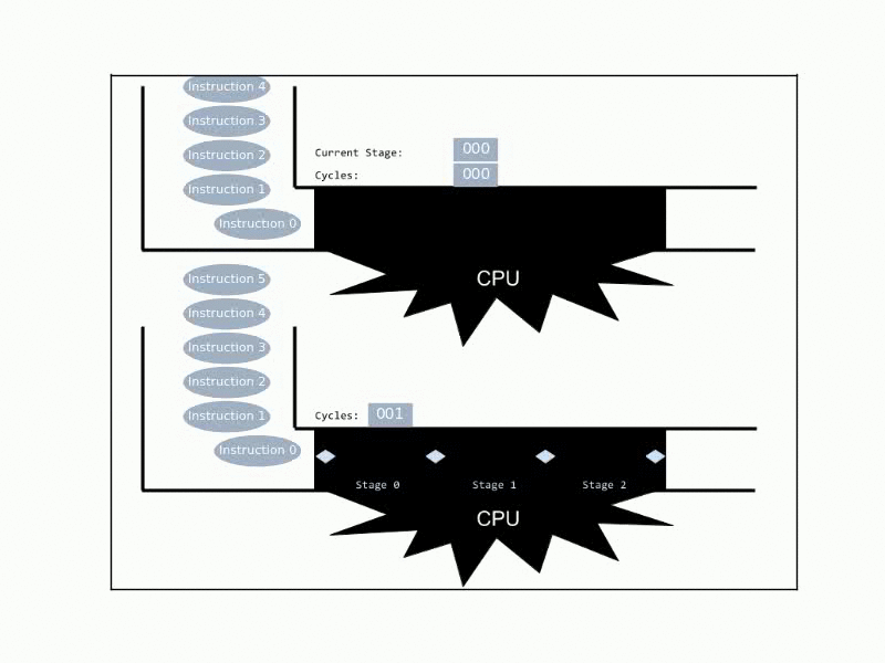
The simplest way to achieve ILP, is by employing pipelines. These are pretty much the computational analogue of manufacturing assembly lines: The CPU breaks an execution of an instruction to a sequence of stages, and at any given time it can handle many instructions simultaneously, given that each is in a different stage. Now, ideally, at any given cycle the CPU completes 1 instruction, even though any given instruction takes multiple cycles to complete.

Real CPUs usually implement much more sophisticated mechanisms of ILP, by introducing duplicated functional units that allow the processor to deal with parallel instructions that are in the same stage. Additionally, CPUs may reorder the instructions, when later quick-to-execute instructions are independent of earlier slow-to-execute instructions.

This requires a real-time management (in hardware) of dependencies between different instructions - which may get pretty complicated pretty fast. There are two major approaches to accomplish this: nowadays superscalar processors are prevalent, but up to not so long ago, a different variation of the idea - called VLIW (for Very Long Instruction Word) - was what all the cool kids got excited about. I won’t get into any of these right now.

Anyway, pipelines in practice can get rather long (10-30 stages). Yet, it’s helpful to simply think about an ideal 6-stages pipeline, with the following stages:

1. F: Fetching the next instruction to be executed from memory.
2. D: Decoding the instruction (here possible dependencies issue are dealt with).
3. I: Issuing, by forwarding the instruction to the appropriate unit, possibly via bypassing (+reading the register file).
4. X: Executing the instruction (i.e. in the ALUs’ gates).
5. M: Memory stage, where memory access is done.
6. W: Writeback, where results are written in the register file.

After an instruction is fetched, the CPU normally goes and fetches the next instruction into the pipeline. That’s where things get messy for branches: if the last instruction was a branch, the CPU doesn’t know what will be the next instruction it should fetch until it makes a lot of progress with the jump instruction.

Even if it was an unconditional branch, the CPU won’t know the destination address before it goes through the D stage if the destination is fixed, or the X stage if the destination is variable. If the CPU had no choice but waiting this long before fetching the next instruction, the overall execution speed of programs would have dropped drastically (in a long-pipelined superscalars, a slowdown by a factor of 5(!) or so wouldn’t be surprising).

Branch predictors to the rescue!

Turns out that programs naturally feature predictable patterns that allow CPUs to accurately guess, for conditional jumps, both the destination and the evaluation of the condition, and keep fetching instructions continuously. If down the road the CPU discovers it guessed wrong, it undos all the incorrect work it mistakenly did, and starts again. That’s an example of speculative execution, and CPUs do this quite a-lot. When they speculate wrong, it’s painful and expensive, so branch predictors must be very accurate, making such events rare. Actually, in modern CPUs an accuracy of less than 98%-99% is considered unpractical.

1.3. Control Structures

Branch prediction is possible because the algorithmical constructs in which branches appear provide regularity and contextual information that make them predictable. We shall now briefly explore the predictability of some common constructs: the if–then–else construct, loops (and nested loops) and function calls. We shall also discuss indirect jumps, which are often used to implement polymorphism (as in C++’s virtual functions) and switch-statements (via jump-tables).

First, loops. Whether the code in the fancy high-level language-de-jour expresses a “while loop”, a “for-each enumeration”, a “map high-order function” or any other fashionable abstraction - at the end, it all looks about the same when it comes down to actual instructions:

loop_label:
    ... ; code
    je loop_label ; Goto loop_label if some condition holds.

... ; more code

In many ways, loop branches are the most easily predictable jumps. Short nested loops commonly obey a pattern in which their branch is taken a fixed number of times, after which it is not taken once (and so on):

 while (long_time) {
     for (size_t i = 0; i < 2; ++i) { /*...*/ } // Yes, Yes, No, Yes, Yes, No, ....
}

And for long loops, the simple strategy of always predict “taken” achieves a low error rate.

But to take advantage of those regularities, the predictor needs a way to identify that a branch instruction is actually a part of a loop. Sometimes the ISA has special instructions to deal with loops (e.g. LOOPxx in x86), which immediately solves this problem (at least after the first time the instruction is decoded). But even if a loop is implemented using regular jumps (either due to lack of support from the ISA, or just because the compiler decided so), it can still be easily identified: it involves backwards jumps. A naive static branch predictor could simple predict that backward-jumps are always taken.

All that was presuming that the destination of the jump is known. Luckily, the destinations of loop-related branches are almost always constants, thus cacheable. After the first time a loop’s branch is encountered, a good strategy for target prediction is to predict the previously taken destination.

Forward-branches, on the other hand, are usually a part of an if–then–else construct. So reason (and empirical tests) suggests they will be taken about 50% of the times. That’s not encouraging, and the best static strategy available here would be to always predict “not taken” (since it’s much easier than predicting “taken”, which then requires a prediction for the destination as well).

Two things can help here. First, is the fact that even if–then–else constructs commonly show some regularity that can be exploited for prediction, as in the following example:

    for (size_t i = 0; i < N; ++i) {
        if (i%3 == 0) { /*...*/ } // Yes, No, No, Yes, No, No, ....
   }

That’s an example of temporal patterns. Secondly, conditional blocks are often dependent, and once some previous conditions are known, other conditions may become highly predictable. Those are spatial patterns:

if (animal.subspecies() == Subspecies::DOG) { /*...*/ }
// ...
if (animal.sound() == Sounds::WOOF) { /*...*/ } // Alway true when the previous condition holds.

In contrast to if-else-thens and loops, function calls usually involve unconditional jumps - so they require only a target prediction. Moreover, most CPUs have specialized instructions for functions (e.g. CALL and RET in x86), which makes their related jumps easily identifiable. So it all seems pretty easy, and indeed it partially is: target prediction for function calls is as easy it gets. The problem starts when the function returns.

By design, functions encapsulate pieces of reusable code and are typically called from many different locations. So when the CPU encounter a RET instruction, the last used target address is useless for predicting the next target address. We later see how CPUs cope with this.

There are also situations in which the target prediction for the function call itself is non-trivial, for example, when the function is polymorphic:

class Animal { virtual void TakeAShower() = 0; };
class Dog : public Animal  { virtual void TakeAShower() {throw NoFreakingWay();} };
class Cat : public Animal  { virtual void TakeAShower() {assert(m_already_clean==true);};
// ...
std::vector<std::unique_ptr<Animal>> animals;
// ...
animals[0]->TakeAShower();

In practice, such function calls involve an indirect jump (also known as “jump register”). Another common usage of indirect jumps are for the implementation of jump- tables. Trampolines, which are thunks that are arranged in the procedure linkage tables used by share libraries that are compiled as a position independent code, may be also implemented using indirect jumps - but they are still perfectly predictable, since the final address of the actual function is constant throughout the execution.

As a final note, it’s useful to know that it’s possible to profile code for branch miss-predictions using valgrind. This profiling is rough and conservative: since the actual branch-predictors in the CPU can’t be queried, valgrind will simulate a branch-predictor while running the code, and it will do so by using prediction methods which are almost certanily less accurate than those actually used by the CPU. The syntax is:

valgrind --tool=cachegrind --branch-sim=yes program

2. Target Prediction

2.1. Branches and Targets

At the beginning of any given cycle, a guess for the location of the next instruction to be fetched must be available. Usually this prediction is easy - at least in theory: if the instruction to be fetched is not a jump, the location of the next instruction is simply the location of the following instruction.

That’s in theory. And while in theory, theory and practice are the same, in practice - well…

In this case there are two issues that complicates even the simplest of cases, where no jumps are involved. Firstly, the CPU does not know in general whether the current instruction is a jump or not until it decodes it. So even if the procedure of dealing with non-jumps was easy, knowing when to apply it - is not.

By itself, that’s not a big problem. The CPU can maintain a cache of addresses that contain jumps, and use it to test whether the instruction it just fetched is a jump. Obviously this cache mechanism would have to be implemented cleverly, since this check must be doable within a single cycle and its space usage is stringently constrained - but that’s also not a problem. The standard data- structure in such cases is a narrow table that is indexed by some of the address’s LSBs and its entries contain “tags”, taken from the address’s MSBs of the last seen jump instruction that was mapped to the entry.

But then, there’s the second issue: the address of an instruction does not provide enough information for accessing its sequential instruction. Not without decoding it. That’s because in many ISAs (even of RISC processors), instructions have a variable length. The naive assumption that instructions are laid in memory such that their addresses form an arithmetic progression is not true in general.

For those reasons, CPUs often perform a partial decoding for instructions in the iCache, before fetching them. This solves both problem. And it has other advantages as well, since there are other types of useful “meta information” that even a partial decoding of instructions may provide - such as whether the instruction is a direct branch, an indirect branch, a function call or a return instruction. Additionally there are more advantages, unrelated to branch- prediction, which won’t be discussed here (e.g. better cache-utilization of μops-based microarchitectures).

Once this is done, and the CPU can identify jump instructions as soon as they’re fetched, target prediction is almost exclusively done by a form of caching, using a data structure called Branch Target Buffer (BTB). The BTB works by tagged-indexing as described earlier (almost: usually it is set-associative), only that it holds an associated value for each of its entries: the target address from the last time the corresponding jump was taken.

2.2. Subroutine Return Stack

Target prediction using the BTB works well in many common cases, including jump- tables and switch-statements with a repeatedly used case, and indirect polymorphic function calls via a pointer which usually points to objects of the same class.

But one very common case in which BTBs perform poorly, is returning from functions, This is an unconditional jump, so only the target prediction plays a role in here - but since functions are commonly being called from many different locations and places, the return address is constantly changing.

To deal with this case, return instructions are treated differently, using a Subroutine Return Stack. This is a special stack, maintained by the CPU, in which the locations of function calls are being stored. This stack is bounded, and when overflowed - the oldest entries are dismissed. This means that long chains of function-calls may reduce performance due to target- mispredictions.

3. Outcome Prediction

3.1. Non-Stationary Bias

The most basic temporal pattern a specific branch may demonstrate is a simple bias. While a general forward branch has about 50% chance of being taken, the branch associated with, say, the condition 1!=0 will be always taken. Of course, most branches are not as degenerated, but most are nevertheless biased.

Going by the book, this is basically an estimation of a Bernoulli distribution, and the naive way to learn the bias of a branch is by counting the times it was encountered and taken and the times it was encountered but not-taken, and use the ratio as an estimation for the bias (possibly after applying Laplace smoothing).

This idea has two major flaws. Firstly, it’s expansive. Keep in mind that those algorithms should be implemented in the CPU and are constrained to execute within 1 cycle. Maintaining 2 counters, and requiring comparison, addition and division is just too much. Secondly, and even more importantly, the distribution of a branch’s behaviour is usually non-stationary. When the code with the given branch is executed in a certain context, the branch may be biased in a very different way than when the code is executed in some other context.

A more appropriate solution is caching: simply saving the last evaluation of the branch, and use it as the next prediction. This requires just 1 bit of storage, no computations, and accounts for non-stationarity. Equivalently, this idea can be also be thought of as using a finite state machine (FSM) with 2 states:

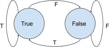
While such FSM requires just 1 bit to implement, which is really good - it suffers from some real drawbacks. For example, it performs poorly on repeated short loops, which are a common pattern (since it always gets wrong the last branch and then again the first branch upon reentry, and for short loops, it means a high mis-predictions ratio). It also performs poorly in some other common scenarios, such as small biases (since each time to predicate will be different than the last time - which is often - two mispredictions will occur).

A generalization of this idea, that overcomes some of those issues, is using larger state machines. For technical reasons, 4 states is the most common FSM used in commercial CPUs. The 4 states a branch can be in, are usually referred to “Strongly True”, “Weakly True”, “Strongly False” and “Weakly False”. A branching predicate that is either in a “Strongly True” or in a “Weakly True” state is predicted as “True” (and the same goes for “False”), but the transition model leads to fewer mistakes in many common situations (e.g. now a nested loop with a short inner loop, has 1 mis-prediction per outer loop instead of 2).

There are two common variations for such FSMs:

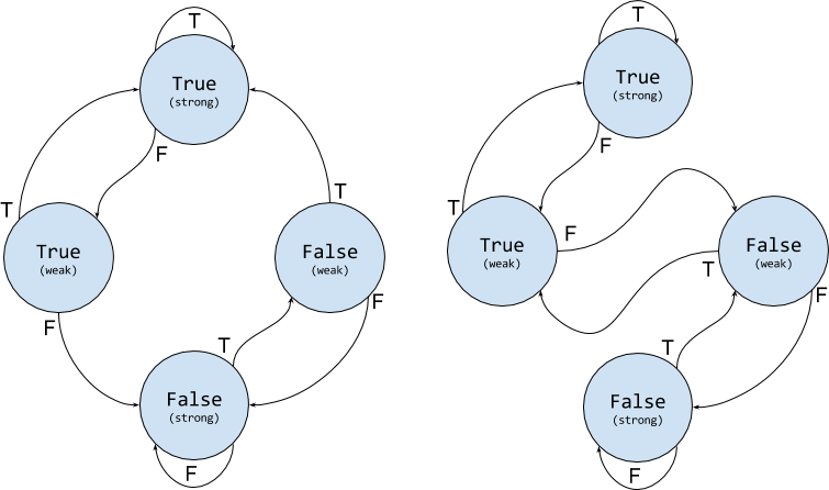
The right FSM is sometimes called 2BC (for 2-bits counter), since it acts as a counter with a 2-bits saturation. In a sense, it keeps balance of “what recently happened more” (with a quota), and uses it for prediction. The idea in the left FSM, is to enter a new prediction state via a strong state. It basically treats consecutive mistakes as a strong signal. The “weak” and “strong” labels can be seen as a “confidence score” for the prediction.

Those two FSMs are very simple and almost identical. But they are a manifestation of two different ideas (a common situation). The right FSM has a strong resemblance to adaptive control algorithms, while the left FSM is the purest form of a state-space predictor.

3.2. Correlating Predictors

Estimation of the (time-varying) bias of a branch is just the very beginning. The next step is to deal with temporal and spatial patterns. For example, a branch that is associated with the condition i%3==0 inside a loop that enumerates using i, will have the pattern FFTFFTFFTFFT... which is highly-predictable.

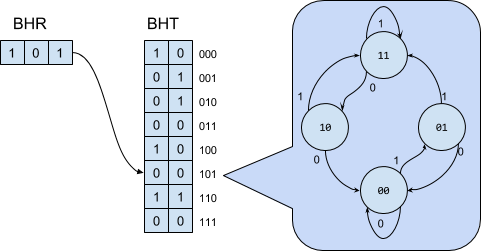
In order to track such patterns, CPUs use a special data-structure. The first element of the data-structure is called “Branch History Register” (BHR), which as its name suggests, is a register (shift-register, actually), that holds the last K evaluations of the branching condition.

Of course, a program has many branches, not just one, and the different branches are not independent. The dependencies between different branch are referred to as “spatial patterns”, and they usually occur due to branches that are near to each others in the code. e.g.

if (x > 0) {
    // do something
    if (x > 5) {
        // do something
    }
}

The second branch is obviously dependent on the first one. The simplest way to take this into account is to make the BHR global. So now the recent evaluations of the K predicates (regardless if they are a multiple evaluations of the same branch, or separate evaluations of different branches) are used.

A better approach is to use a local branch-predictor for each branch. This can be done by maintaining M separate BHTs, and use the address of the predicted branch to choose the BHT that learns this branch. Then the BHR is used to index to correct BHT as usual. The result if called “Two-Level Branch-Predictor”. Of course, it is not possible to keep a BHT for any possible instruction of a given program (that would require way to much space). Instead some of the LSBs of the address are used as an index to the correct BHT, and only about 100 BHTs are used.

This can be taken further, by maintaining a separate BHR for each branch. Such a table of branch-history registers is called “Pattern History Table” (PHT), and the resulting predictor is called “Generalized Two-Level Branch- Predictor”:

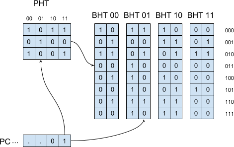
Note, this time each branch is predicted using its own local history - and spatial patterns are not taken into account.

There exist several other variations on this theme. For example, the Pentium Pro (circ 1995) used a 2-bits BHR and 4 BHTs whose entries maintained 2-bits counters.

3.3. Shared Biases

The two-level branch-predictors described above are wasteful: for most branches, most patterns are never encountered, and most of the dedicated bits in the BHRs remain unused. To mitigate this, CPUs often reuse the same structure of bias- estimators (the FSMs from the first section) for all the branches. That allow for the implementation of branch-predictors that can deal with very long patterns using 2 or 3 bits FSMs, that requires only a few kilobits of storage.

Such shared-predictors come in two flavours. The first one, sometimes called PShare (for “private history, shared FSMs”) is similar to the generalized two-level predictor from earlier in that it considers the temporal patterns of each branch separately, and does not take into account spatial pattern involving several different branches. The idea is to “mesh together” the history-pattern of the current branch with some bits of its address (usually simply by xoring) to index into a BHT. Since each entry of the BHT takes 2 or 3 bits, it can be large, and collision are rare:

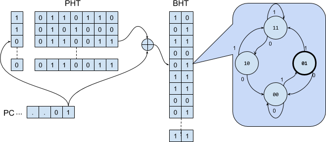
The second flavour, GShare (for “global history, shared FSMs”, of course), uses a global BHR instead of a BHT. So it exploit spatial patterns, but is not very efficient when it comes to local temporal patterns (especially long ones).

3.4. Ensembles and Hierarchies

What really brings branch predictors to their best performance is the use of stacking. This allows them to exploit both private histories and spatial patterns as the context dictates. Combining different types of predictors has many other advantages as well: CPUs can assign simple predictors that perform well on most cases to most branches, but keep some complicated or specialized predictors and assign them to hard-to-predict branches.

The simplest form is a Tournament Predictor, in which the CPU has both a PSHare predictor and a GShare predictor, together with a third meta-predictor (often referred as “a choice-predictor”) that decides for each branch, whether it should be predicted using the PShare or the GShare predictor. The choice- predictor is essentially just a BHT whose different entries are 2 or 3 bits FSMs

• one per local branch - that decides how to predict their corresponding branch:

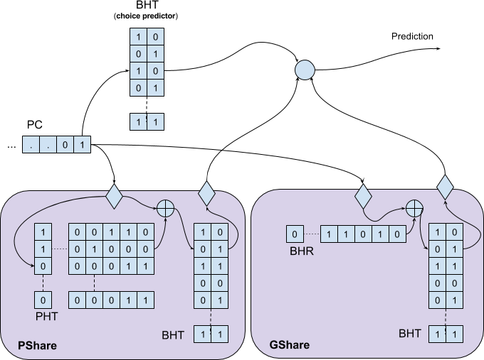
A special care should be taken with the training of tournament predictors. The choice predictor is basically a “bias estimation” finite-state-machine per- branch, and at each iteration only 1 concrete predictor (either the PShare or the GSHare) is updated based on the actual branch outcome, while the choice- predictor itself is updated base on the success of the concrete predictor (so if both are right or both are wrong, nothing changes - but if one is right and the other is wrong, a bias is strengthened). The catch is, that since the true outcome is known only late in the pipeline, and in the meanwhile more predictions are usually made - the global predictor is speculatively updated, but restored later on mispredictions.

The idea is originated with the Alpha 21264 processor (i.e. it’s around since 1996), and it’s still more-or-less the prevalent design of branch predictors. But newer CPUs takes things further. The main addition introduced by modern predictors, is an hierarchical architecture in which specialized predictors can be integrated (e.g. a special counter-based predictor for loops).

Hierarchical predictors take advantage of the fact that typically many branches display simple and regular behaviour: they are almost always have the same outcome. So for those branches, a very simple branch-predictor can be used (i.e. 1 bit cache). Since such predictors are very cheap, many such predictors can be maintained simultaneously, and many different branches can be tracked. More complicated branches are dealt with using a more complex predictors (e.g. 2-bits FSMs), which are more expensive but rarer, and only the most complicated branches are predicted using a tournament predictor

• which now is required to deal with much fewer branches, hence can exploit more complex patterns.

This is, for example, the type of prediction algorithm that is implemented in Intel’s Pentium M CPU (from 2003). By default, it predicts branches using a 2-bit FSMs. But it also maintains a PShare and a GShare predictors. Each branch is mapped to all 3 predictors using its address’s LSBs, and a tag-check in the PShare and GShare predictors (using some of its address’s MSBs) is used to determine if they should handle it. A priority is given to the GShare, then (if the branch is not in the GShare predictor) to the PShare, and then (if the branch is not in the PShare predictor), the 2-bit FSM from the BHT is used for prediction. A branch that is predicted poorly is “moved up” the hierarchy. Intel’s Core i7 also implements an hierarchical predictor, and incorporates a specialized counter-based loop predictor in it.

Those are the types of predictors that finally achieve an accuracy of over 99%.

4. Conclusion

The problems imposed by branches are a fundamental obstacle in the way of high performance computing. Luckily, learning algorithms offer a very practical solution.

CPUs are using a combination of costume data-structures, cheap hashing techniques and finite-state machines to implement suitable algorithms, instead of the “default” solutions such as Q-Learning, Value and Policy iterations or Hidden Markov models. By doing so, they achieve a stunning accuracy under the most stringent constraints.

Variations of those methods are highly applicable for integrating learning algorithms in general embedded systems or real-time computing, or for speeding up the training time of expensive models.