The Name of The Rose

Many ideas in machine learning came up independently in different contexts, and it's not uncommon to have multiple terms for the same concept. Those instances are usually dismissed as nuisance; after all, a rose by any other name, et cetera. Indeed, often this is just a matter of nomenclature, and with time conventions form, and some terms disappear while others acquire universal meaning. But sometimes the distinction is not as superficial as it may seem.

Recently I encountered such a situation, in which while explaining someone a term I used, it became clear that this person was already familiar with the concept under a different name. But what initially looked like nothing more than a confusing lingo, turned out to be of fundamental significance.

An electrical engineer is facing the task of building an active noise-canceller for cellular phones: a device that transmits the speaker's voice while omitting the environmental noise. This can be done using an additional directional microphone to record the environment, and a filter that subtracts it from the recordings of the main microphone used to record the speaker.

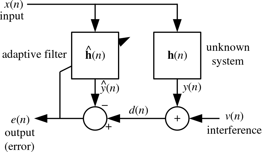
Since the filter's transfer function should vary in time, in response to the unpredictable environmental noise, an adaptive filter is required. The simplest such filter is the so-called "least mean squares" (LMS) filter. Here's its block diagram (taken from Wikipedia):

Naively implementing it in software is straightforward:

In the context of noise cancellation, the engineer applies it backwards, by using the noise signal $r_1(t)$ to remove the speech-signal $v(t)$ from the noisy speech-signal $v(t)+r_2(t)$ (note that $r_1(t)\approx r_2(t)$, but they are not equal since they were recorded using different microphones in different locations).

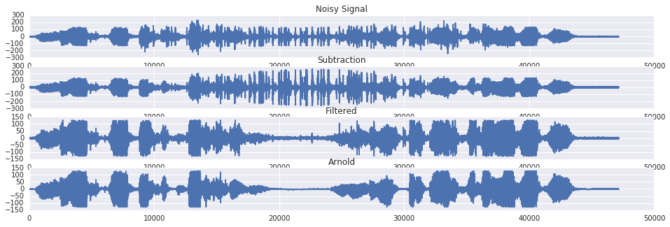
As a demonstration, consider the canonical example of Arnold Schwarzenegger trying to make a phone call while watching a bear riding a motorcycle:

A statistician is hired by a retail company for the task of minimizing delivery times from their warehouse to their stores. There are multiple routes between the warehouse and any of the stores, and the traffic in those routes erratically changes during the day. For simplicity, let's focus on the case of 1 store with 2 possible routes.

There is some potentially useful information available, such as reports from navigation applications (e.g. Waze) and a-priori estimations of the current traffic based on the time (e.g. the notorious traffic jams of Wednesday mornings) - but it's not clear how to factor it into a decision, due to the instability of the traffic patterns. For example, sometimes traffic jams tend to clear up quickly and current reports should carry little weight relative to the day and time, and sometimes they're persistent and reports should be taken very seriously.

This hints towards online learning: constantly updating the decision rule based on its recent performance. The perceptron is the simplest online classification algorithm. It is very roughly modeled after a biological single neuron (the McCulloch–Pitts model). It may either "fire" or "hold", and the decision is based on whether its weighted accumulated input is crossing a threshold. Schematically:

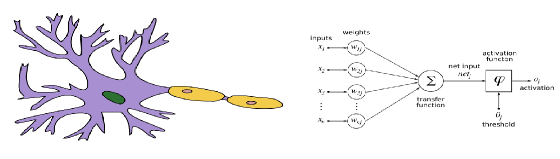
The weights are learnt in a supervised manner using an algorithm known as "the perceptron's update rule", which is applicable as an online algorithm. The update rule is rather heuristic: if there's no error, keep the weights; otherwise, change the weight of each input in proportion to its magnitude, in the opposite direction of the error. If "fire" is represented by 1 and "hold" by 0, the rule is simply $w_{i,t+1}\leftarrow w_{i,t}+\delta(y_t-\hat{y}_t)x_i$.

Say the statistician has 4 sources of information: $R_1, R_2 \in[0,1]$ are the current reports regarding route A and route B respectively (0 means the route is clear and 1 means it's jammed), and $A_1, A_2\in[0,1]$ are the current (periodic) time-based estimations of the traffic in the routes:

The decision is going to be based on the difference between the current traffic estimations based on real-time repotrs $R_1-R_2$, and the difference between the current traffic estimations based on the current time and date $A_1-A_2$:

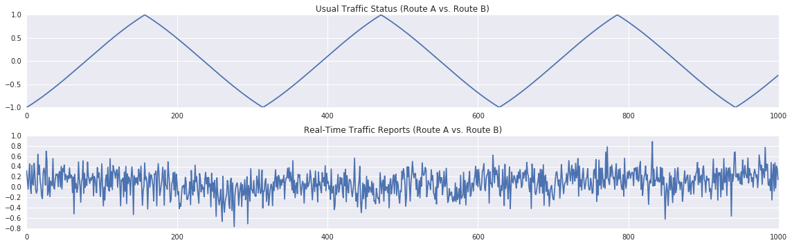
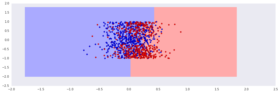
Due to the temporal dynamics, a stationary classifier is unlikely to work, and the classes aren't linearly separable:

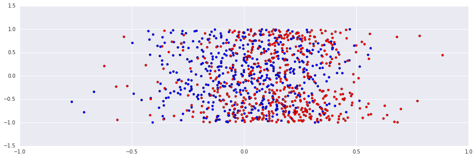
On the other hand, the online learning algorithm is adaptive to the temporal structure, and works rather well:

A consumer product company starts a new campaign over the internet, and it needs to decide how much it is worth paying for serving its new ad. The decision should take into account the potential viewer demographics (say, age and economic status), and the evaluation must somehow mitigate the fact that the impact of the ads is indirect and delayed: it's impossible to relate a specific sale with a specific viewing of an ad. Moreover, the effectiveness of the ads is likely to vary over time.

An algorithm designer is assigned with the task of writing the engine that interacts with the demand-side platform. The standard framework for constructing a policy that maximizes long-term utilities based on observed immediate rewards is Temporal Differences. In the current simplified setting, the policy should be based on a linear function of an "age signal" $x_t\in[0,1]$ (where 1 means a viewer in his twenties, and 0 means the viewer is either much younger or much older), and a "economic status" signal $y_t\in[0,1]$ (where 1 means "spendthrift").

At each time-step, the engine receives a reward $r_t$, which measures the flow of incomes from sales. Of course, the value of $r_t$ is the noisy result of previous exposure to ads, and has nothing to do with the decision made by the engine at time $t$.

Dealing with (potentially infinite) sequences of rewards leads to the idea of "discounted rewards" (with a discount factor $\gamma$). So the utility at time $t$ is $U(x_t,y_t)=E[\sum\gamma^{i-1}r_{t+i}|(x_t,y_t)]$, and the engine maintains an estimation $\hat{U}_t\approx U$, and iteratively updates it based on his observations.

Discounting can be understood in several ways: it can be derived axiomatically by specifying some reasonable properties of temporal preferences (c.f. Koopmans), or it can be seen as a way to incorporate infinite horizons with random stopping times, or finally, it can be justified economically by considering the usual stories about the risk that is associated with future incomes, or about the "hypothetical losses" of potential profits that could be obtained by investing the said income in the present.

For example, say that in time $t-1$ the engine observed $(x_{t-1},y_{t-1})$, rewarded $r_{t-1}$ and served an ad based on the estimation $\hat{U}_{t-1}(x_{t-1},y_{t-1})=u_0$. Then in time $t$ it observed $(x_t,y_t)$, and experienced an immediate reward $r_t$. So one option the engine may employ, is to update $\hat{U}_{t}(x_{t-1},y_{t-1})=\alpha(r_t+\gamma\hat{U}_{t-1}(x_t,y_ t)-\hat{U}_{t-1}(x_{t-1},y_{t-1}))$ and $\hat{U}_{t}(x,y)=\hat{U}_{t-1}(x,y)$ for $(x,y)\neq (x_t,y_t)$ (where $\alpha$ is the learning rate).

This is knowns as $\mathrm{TD}{(0)}$ rule, and it's a special case of the $\mathrm{TD}(\lambda)$ algorithm which I won't discuss here ("TD" stands for temporal differences). In this case, $\hat{U}_t(x,y)=\omega_1x+\omega_2y$, so the update rule should be applied to update the weights $(\omega_1,\omega_2)$. This can be naturally done by $\omega_1\leftarrow\omega_1+\alpha (r_t+\gamma\hat{U}_{t-1}(x_t,y_t)-\hat{U}_{t-1}(x_{t-1},y_{t-1})) x$ (and the same applies for $\omega_2$).

Here a simulation of the situation described above:

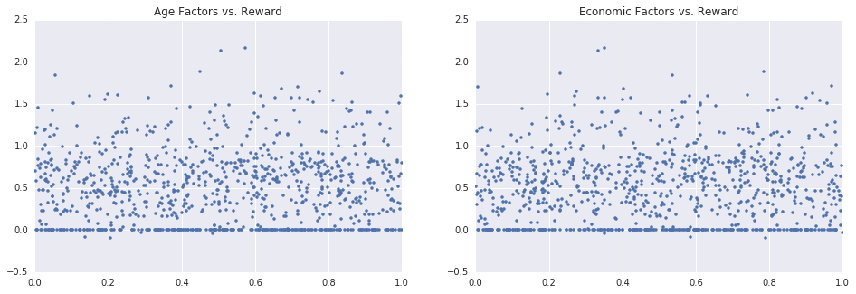
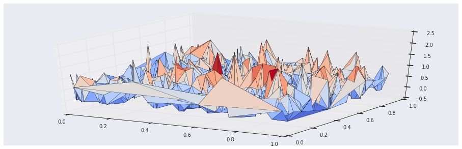
Since the profits from an ad are both delayed and stochastic, at any given time there will be no relation between the current user, and the current reward - which makes it hard (impossible?) to learn a good decision rule by using supervised learning algorithms:

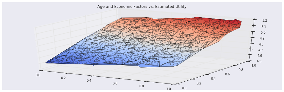
On the other hand, the temporal differences algorithm recovers the true utility associated with the users:

The above are three completely different formulations, motivated by completely different scenarios. But at the end, the essentially same algorithm was derived: it's the same iterative scheme, with almost identical update rules. A clear case of convergent evolution.

The obvious suggestion is: let's just call that algorithm ILT ("Iterative Linear Thingie") and forget all those obscure terms we introduced ("lms", "perceptron", "temporal differences"...).

Should we? The answer depends on the price. Adopting the ILT suggestion will obscure the different perspectives that led to the resulting algorithms, and the price is losing those nuances. This could be perfectly reasonable had those perspectives ran their course, but this is hardly the case: generalizations of this ILT algorithm are utterly unalike when guided by each of those different points of view.

For example, the LMS filter may be generalized to other adaptive filters, such as the Kalman filter which is commonly used in varied situations, from trajectory optimization to econometric smoothing. The perceptron may be generalized to other classification algorithms (e.g. logistic regression, support vector machines and feedforward neural networks). And the temporal differences algorithm is a basis for many algorithms (e.g. Q-learning) in optimal control and autonomous agents, and it can be used to train computers to play backgammon or super-mario better than you can.

None of those generalizations is obvious by considering the ILT alone. But all of them are quite natural as a development of the ideas that led to the ILT in the first place, from the 3 different starting points.

It's worth pointing out that this phenomenon is not unusual, and definitely not limited to machine learning. For example, in elementary calculus an "integral", an "area under the curve" and an "anti-derivative" are pretty much 3 names for the same concept, originated from 3 different perspectives (namely: analytic, geometric and algebraic). But generalizations of this "same concept" take completely different turn when developed from each of those perspective (respectively: differential forms, measures and differential equations).

Regarding the title, wikipedia says: "Eco has stated that his intention was to find a 'totally neutral title'... [it] 'came to me virtually by chance'".