The Generative-Discriminative Fallacy

It is customary to categorize predictive algorithms as either "generative" or "discriminative". Denoting by $Y$ the target and by $X$ the observable, discriminative algorithms are those that model the conditional distribution $P(Y|X;\theta)$ and generative algorithms are those that model the joint distribution $P(X,Y|\theta)$) (note that this entire discussion presumes a probabilistic perspective on predictive tasks).

Prima facie, the distinction seems senseless: the conditional distribution and the joint distribution are intimately related via Bayes theorem $P(Y|X)=\frac{P(X,Y)}{P(X)}=\frac{P(X|Y)P(Y)}{P(X)}$, and for prediction, $P(X)$ is in effect unnecessary since $\mathrm{argmax}_YP(Y|X_0)=\mathrm{argmax}_Y\frac {P(X_0,Y)}{P(X_0)}=\mathrm{argmax}_YP(X_0,Y)$.

Still, the situation is fundamentally asymmetric: many different joint distributions $P(X,Y)$ admit the same conditional distribution $P(Y|X)$. Hence common sense (and even better, Vapnik) suggests that discriminative models are preferable for prediction. After all, they model the problem directly, while generative models require solving "a more general problem as an intermediate step".

This is somewhat true. For example, one may assume the generative model $X|y_i \sim \mathrm{Poisson}(\lambda_i)$ and $Y \sim \mathrm{Bernoulli}(p)$ and train it using MLE. If things go terribly wrong, and in reality $(X|Y=y_i) \sim \mathcal{N}(\mu_i,\Sigma)$, the classification algorithm will embarrassingly fail. On the other hand, under either of those assumptions, training the model discriminatively amounts to optimizing the appropriate loss of the objective $P(Y|X;\beta)=(1+\exp{(-\beta^TX)})^{-1}$. Had this have been done, the classification algorithm would have worked in both cases.

So it looks as if the distinction is not senseless after all.

Or is it?

But that's wrong: generative-discriminative pairs typically consist of two completely different models. The procedure for making such pairs is something along these lines: start with $P_1(X,Y|\theta)$, derive $P_2(Y|X,\theta)$, and take as the generative counterpart the model $\hat{Y}_G=\mathrm{argmax}_YP_1(X,Y|X,\hat{\theta}_G)$ where $\hat{\theta}_G:=\mathrm{argmax}_\theta P_1(X_\text{train},Y_\text{train}|\theta)$, and as the discriminative counterpart the model $\hat{Y}_D=\mathrm{argmax}_YP_2(Y|X,\hat{\theta}_D)$ where $\hat{\theta}_D:=\mathrm{argmax}_\theta P_2(Y_\text{train}| X_\text{train},\theta)$.

Those are clearly two different probabilistic models, and the central point is this: if the assumptions underlying the generative model $P_1$ (which also underly $P_2$) actually hold, then $P_1$ is optimal, and will outperform any other model (including $P_2$). The statement "discriminative models have lower asymptotic error" is outright false in such generality. It's true only in a "distribution free" sense. Any advantage discriminative models may have, is due to misspecifications of the probabilistic models from which they were derived.

This brings me to the second misconception: robustness. The aforementioned paper discusses the family $\mathcal{H}$ of linear classifiers $\mathcal{X}\mapsto\mathcal{Y}$ where $\mathcal{X}=\{0,1\}^n$ and $\mathcal{Y}=\{\text{y}_0,\text{y}_1\}$, and concludes that reasonable generative-discriminative pairs ($h_G$, $h_D$) asymptotically satisfy $\epsilon(h_D)\le\epsilon(h_G)$ where $\epsilon(h):=P_\mathcal{D}(h(x)\neq y)$ is the generalization error with respect to the arbitrary distribution $\mathcal{D}$ over $\mathcal{X}\times\mathcal{Y}$. This is a trivial consequence of "modeling the problem directly".

Then it gives an explicit example: a naive Bayes classifier as a generative model, and a logistic regression as its discriminative adjoint. The derivation of this pair is simple: in the normal case, the naive Bayes assumption $P(\mathcal{X}|\mathcal{Y}=\text{y}_i) \sim \mathcal{N}(\mu_i,\Sigma)$ implies that $\ln{\frac{P(\mathcal{Y}=\text{y}_0|\mathcal{X})}{P(\mathcal{Y}=\text{y}_1| \mathcal{X})}}\propto(\sum\frac{(x_i-\mu_{i,\text{y}_1})^2}{2\sigma_i^2}-\sum\frac{ (x_i-\mu_{i,\text{y}_0})^2}{2\sigma_i^2})=\sum{\alpha_ix_i}+\beta$. Thus from the robustness point-of-view, estimating the coefficients $\alpha_i$ and $\beta$ by minimizing the classification error and using the resulting classifier instead of naive Bayes is a great idea, isn't it?

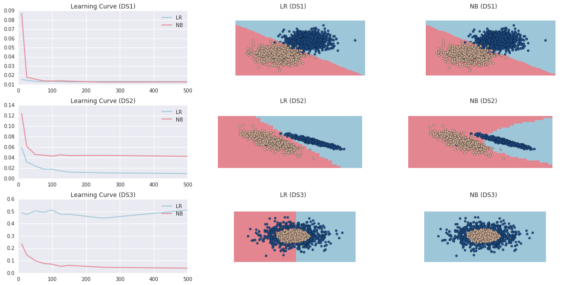
It should be emphasized that the failure of the logistic classifier above in the linearly inseparable setting, is not due to the fact that it's a "discriminative model". It fails because the derivation of the logistic training algorithm from the naive Bayes model, was crucially based on the assumption that the covariances of the distributions $P(\mathcal{X}|\mathcal{Y}=\text{y}_0)$ and $P(\mathcal{X}|\mathcal{Y}=\text{y}_1)$ are the same.

When this assumption is violated, the logarithm of the odds ratio is no longer a linear function of the observations. Instead all we can say is that $P(\mathcal{Y}=1|\mathcal{X})=\frac{1}{1+e^{-2F(\mathcal{X})}}$ where $F(\mathcal{X}) =\sum\frac{(x_i-\mu_{i,\text{y}_1})^2}{2\sigma_{i,\text{y}_1}^2}-\sum\frac{ (x_i-\mu_{i,\text{y}_0})^2}{2\sigma_{i,\text{y}_0}^2}$. This model can still be trained as a discriminative model! It's just no longer a logistic regression.

When comparing a regular generative naive Bayes model with such a proper "discriminative naive Bayes" (which is very much not equivalent to a logistic regression), the trade-off mentioned above indeed holds: the discriminative algorithm has a lower asymptotic error, while the generative algorithm converges faster to its asymptotic performance. But the situation is clearly subtle.

Continuing with the example above, let's fuse naive Bayes and logistic classifiers. Originally, I think such a model was first introduced in the context of text classification, where documents might have different regions with varying importance with respect to the classification task (e.g. a title, an abstract and a body). The method used, involved assigning each region an "importance weight" $\theta_j$ and modify accordingly the usual naive Bayes decision rule -

$$\sum_j{(\theta_j\sum{\ln(\hat{P}(X_i^j=x_i|Y=1))}})+\ln(\hat{P}(Y=1))\ge\sum_j {(\theta_j\sum{\ln(\hat{P}(X_i=x_i|Y=0))}})+\ln(\hat{P}(Y=0))$$

The estimations for $\hat{P}$ were obtained by training a separate (generative) naive Bayes on each region, and the weights $\vec{\theta}$ were discriminatively obtained by utilizing a jackknifeish "leave-one-out" strategy. Nicely, the model could be reformulated to look like a logistic-classifier: $\hat{P}(y=1|x)=\frac{1}{1+\exp({-(\alpha+\sum{\theta_j\beta_j})})}$ with $\alpha=\ln\frac{\hat{P}(y=1)}{\hat{P}(y=0)}$ and $\beta_j=\ln{\frac{\hat{P}(x_j|y=1)}{\hat{P}(x_j|y=0)}}$.

Let's pause and consider the interplay between generative and discriminative algorithms in this model: intuitively, each region is treated as if it were internally conditionally independent, where the signals from different regions could be non-neglectably dependent. Statistically, the Neyman–Pearson lemma offers an interpretation: each of the $\beta_j$'s values is a function of the significance given by a likelihood ratio test performed on a certain projection of the features-space. Then a logistic classifier is used as a meta-model that considers those dependent signals as competing indicators regarding the label.

Obviously, the discriminative likelihood $\mathcal{L}_D(\theta)=P(Y|X,\theta)$ requires access to target values. But so does the generative liklihood $\mathcal{L}_G(\theta)=P(X,Y|\theta)$. Going back to Bayes theorem (actually, just to the definition of conditional probability), we see that $P(X,Y|\theta)=P(Y|X,\theta)P(X|\theta)$. That's almost what we're looking for: a decomposition of the full model into a discriminative model and a separate generative model of the features space. All that is left is to emphasize the separation: $P(X,Y|\theta_1,\theta_2)=P(Y|X,\theta_1)P(X|\theta_2)$. This is indeed the required unified form.

It becomes clear from a Bayesian perspective. Write $P(X,Y,\theta_1,\theta_2)=P(\theta_1,\theta_2)P(Y|X,\theta_1)P(X|\theta_2)$, and note: the constrain $\theta_1=f(\theta_2)$ restores the generative model as a special case, and the constrain $P(\theta_1,\theta_2)=P(\theta_1)P(\theta_2)$ restores the discriminative model as a special case (since then $P(X,Y,\theta_1,\theta_2)=P(\theta_1)P(Y|X,\theta_1,\theta_2)$).

In between it's possible to interpolate the model freely and smoothly on the generative- discriminative spectrum (no longer a dichotomy). e.g. we may use $P(\theta_1,\theta_2)\propto P(\theta_1)P(\theta_2)\sigma^{-1}\exp{(-||\frac{ \Theta_2-\Theta_1}{\sigma}||^2)}$ and control the "generativity" of the model by modifying $\sigma$.