Learning Dynamical Systems
1. Motivational Speech
Quantification of qualitative concepts is a big part of data-science. Typically, this translates to an identification of a specific model from a family of qualitatively-equivalent models (e.g. starting by knowing that $x$ and $y$ are proportional, and ending by pinpointing the relation $y=\frac{1}{3}x$).
Qualitative models come in many shapes and varieties: functional, stochastic, agent-based, geometric, relational and so on. When the observables have temporal or spatial structure, differential equations are the default approach.
For example (warning: extreme simplification ahead), consider wages $\omega(t)$ and employment level $e(t)$. The central bureau of statistics constantly estimates both $\omega(t)$ and $e(t)$, and would like to predict for obvious reasons the employment level few months ahead. Knowing nothing about nothing, they might think of using some linear model for this predictive task (something in the spirit of $e(t+1\text{YEAR})\approx\alpha\omega(t)+\beta e(t)$), which is likely to work very poorly.
Alternatively, they might try to model the situation a bit more accurately. At times when the employment is nearly full, the bargaining power of the employees increases, and with it their wages. In turn, higher wages shrink the employers profit margins, and the incurring risk leads to less employment. So amusingly, as Goodwin has noted at the sixties, the economic system of wages and employment is very similar to a biological ecosystem of predators and preys. Such systems can be modeled using the Lotka–Volterra Equations.
Those are non-linear and first-order ODEs, that model the dynamics of the prey population $e(t)$ and the predators population $\omega(t)$ by a family of differential equations, parameterized by $\Theta=(\theta_1,\theta_2,\theta_3,\theta_4)$:
The model is straightforward: The rate of growth of the prey population is simply proportional to their population size, with proportion that decreases linearly as the predators population increases. Similarly, the rate of reduction of the predators is proportional to their population size, with proportion that increases linearly as the prey population increases. The solutions for the model are generally well-behaved, but don’t have a simple closed-form formula.
In [1]:
def lotka_volterra_system(x, t, theta):
    dx1dt = theta[0]*x[0] - theta[1]*x[0]*x[1]
    dx2dt = -theta[2]*x[1] + theta[3]*x[0]*x[1]
    return [dx1dt, dx2dt]

def lotka_volterra_simulation(theta, xi, times, noise_mu=0.0, noise_sigma=0.05):
    samples = scipy.integrate.odeint(lotka_volterra_system, xi, times, args=(theta,))
    noise = np.random.normal(noise_mu, noise_sigma, size=(len(times), 2))
    return pd.DataFrame(index=times, data=samples+noise, columns=['prey', 'predator'])
Knowing the specific parameters $\Theta$ corresponding to the system at hand, provides a good way to predict future values via simulation:
In [2]:
def predictive_simulation(data, theta, steps):
    N = len(data)
    prediction_prey = np.zeros(N)
    prediction_predator = np.zeros(N)
    for i in xrange(len(data)):
        prediction = scipy.integrate.odeint(lotka_volterra_system, data.values[i, :],
                                            data.index.values[i:i+steps+1], args=(theta,))[-1]
        prediction_prey[i] = prediction[0]
        prediction_predator[i] = prediction[1]
    return prediction_prey, prediction_predator
In [3]:
THETA, XI, steps = [0.5]*4, [1.0, 0.1], 5

train = lotka_volterra_simulation(THETA, XI, np.linspace(0, 50, 100))

model = sklearn.linear_model.LinearRegression(fit_intercept=False)
model.fit(train.values[:-steps, :], train.values[steps:, 0])

test = lotka_volterra_simulation(THETA, XI, np.linspace(0, 50, 100))

lm_prediction = model.predict(test.values[:-steps, :])
sim_prediction, _ = predictive_simulation(test, THETA, steps)

target, = plt.plot(test.values[steps:, 0], '--k', label='target')
linear, = plt.plot(lm_prediction, 'b', label='linear prediction')
simulated, = plt.plot(sim_prediction, 'r', label='simulated prediction')
plt.legend(handles=[target, linear, simulated])
Out [3]:
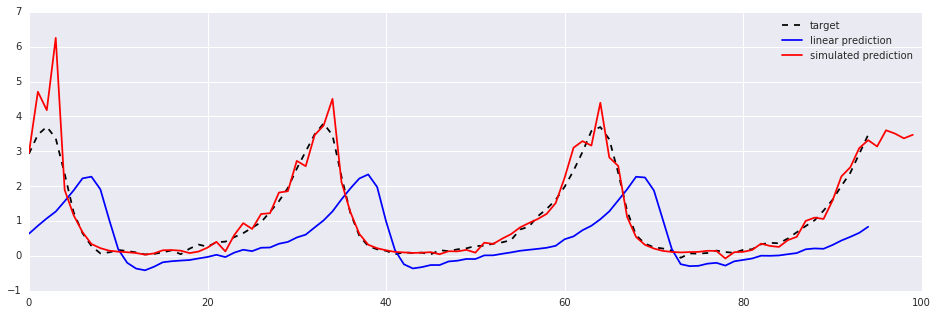
So this leads to the central question of this post: how can the parameters $\Theta$ be estimated?
This is an interesting topic, requires balancing trade-offs regarding statistical considerations, numerical accuracy and computational efficiency. The following is based on a paper by Dattner and Gugushvili, and will deal with the general case. The Lotka-Volterra equations will be used as a running example ($x_1$ will denote the prey, and $x_2$ the predators).
2. Nonlinear Least-Squares
Given a noisy measurements of the prey population $y_1(t)$ and the predators population $y_2(t)$ for some time points $t\in T:={t_0,t_1,t_2,…,t_n}$, the simplest way to estimate $\Theta$ is by “brute-force”: for any hypothetical values $\hat{\Theta}$ of the parameters, the resulting population $x_1(\hat{\Theta}, t)$ and $x_2(\hat{\Theta}, t)$ induced by the model at times $t\in T$ can be calculated by numerically solving the corresponding initial- value problem (e.g. via multistep or Runge–Kutta methods). Thus it’s possible to estimate $\Theta$ by minimizing the error term -
The advantages of this approach is that it’s easy to implement, and statistically well-behaved (apparently, the result is an efficient estimator which is $\sqrt{n}$-consistent).
The problem is that it’s computationally inefficient and numerically dubious. This is because the optimization procedure (typically some gradient descent method) has to repeatedly solve numerically the differential equations (hence the computational inefficiency), and the combination of noisy observations with the approximation errors inherent in the numerical integration may direct the optimization toward a spurious local minima.
In [4]:
def lotka_volterra_LSE_objective(observations):
    def mean_squared_error(eta):
        theta, xi = eta[:4], eta[4:6]
        expected = scipy.integrate.odeint(lotka_volterra_system, xi, observations.index.values, args=(theta,))
        return np.mean(np.square(expected-observations.values))
    return mean_squared_error
In [5]:
THETA, XI = [0.5]*4, [1.0, 0.1]

train = lotka_volterra_simulation(THETA, XI, np.linspace(0, 20, 100))
err = lotka_volterra_LSE_objective(train)
estimated_theta = scipy.optimize.minimize(err, x0=[0.25]*4+[0.5, 0.5],
                                          method='CG', options={'maxiter':1000}).x


print 'Theta: '
print '\t Actual:    ', THETA
print '\t Estimated: ', estimated_theta[:4]
print 'Initial Value: '
print '\t Actual:    ', XI
print '\t Estimated: ', estimated_theta[4:6]
Out [5]:
Theta:
   Actual:     [0.5, 0.5, 0.5, 0.5]
   Estimated:  [ 0.50484547  0.50334676  0.49495745  0.49846957]
Initial Value:
   Actual:     [1.0, 0.1]
   Estimated:  [ 0.98537009  0.10216832]
3. Smooth-and-Match
Another borderline-obvious appraoch for solving the same problem, is utilizing smooth interpolation and numerical differentiation to learn $\hat{x_i}(t)$ and $\frac{\partial}{\partial t}\hat{x_i}(t)$ directly from the measurements $y_i(t)$, holding them fixed, and estimating $\Theta$ by solving the resulting regression problem (i.e. by minimizing $\int||\frac{\partial}{\partial t}\hat{x_i}(t)-F(\hat{x_i}(t),\Theta)||dt$).
Of course, both smooth interpolation and numerical differentiation can get rather tricky in practice, but still - this method is as simple as it gets, and computationally fast: it does not involve any integration what-so-ever. The alleged down-side is that the resulting estimator is not statistically efficient. The practical implications of this fact is likely to vary from application to application.
In the example below, the interpolation is done via quadratic splines:
In [6]:
def lotka_volterra_SME_error(interpolated_x1, interpolated_x2, numerical_dx1dt, numerical_dx2dt, times):
    def L2_error(theta):
        expected_dx1dt, expected_dx2dt = lotka_volterra_system((interpolated_x1, interpolated_x2), times, theta)
        return np.mean(np.square(expected_dx1dt-numerical_dx1dt)+np.square(expected_dx2dt-numerical_dx2dt))
    return L2_error
In [7]:
def interpolate_x(observations):
    times = observations.index.values
    spl_x1 = scipy.interpolate.UnivariateSpline(times, observations.prey.values, k=2, s=0)
    spl_x2 = scipy.interpolate.UnivariateSpline(times, observations.predator.values, k=2, s=0)
    interpolated_x1 = spl_x1(times)
    interpolated_x2 = spl_x2(times)
    interpolated_dx1dt = spl_x1.derivative()(times)
    interpolated_dx2dt = spl_x2.derivative()(times)
    return interpolated_x1, interpolated_x2, interpolated_dx1dt, interpolated_dx2dt
In [8]:
train = lotka_volterra_simulation([0.5]*4, [1.0, 0.1], np.linspace(0, 20, 50))
interpolated_x1, interpolated_x2, interpolated_dx1dt, interpolated_dx2dt = interpolate_x(train)
In [9]:
err = lotka_volterra_SME_error(interpolated_x1, interpolated_x2, interpolated_dx1dt, interpolated_dx2dt, train.index)
estimated_theta = scipy.optimize.minimize(err, x0=[0.1]*4, method='L-BFGS-B').x

print 'Theta: '
print '\t Actual:    ', THETA
print '\t Estimated: ', estimated_theta[:4]
print 'Initial Value: '
print '\t Actual:    ', XI
print '\t Estimated: ', interpolated_x1[0], interpolated_x2[0]
Out [9]:
Theta:
   Actual:     [0.5, 0.5, 0.5, 0.5]
   Estimated:  [ 0.49207082  0.49339354  0.4920194   0.49526578]
Initial Value:
   Actual:     [1.0, 0.1]
   Estimated:  0.98565251968 0.117149797904
4. Accelerated Least Squares
The idae behind the Accelerated Least-Squares method is deceivingly simple: quickly obtain an initial guess $\hat{\Theta}_0$ for the parameters using Smooth-and-Match (SME), and use it as the starting point of a Least-Squares optimization.
But somehow, due to some obscure black-voodoo I do not yet understand (again, see the paper), a mere single Newton-Raphson iteration is enough to obtain an estimator which is statistically as-good as the one given by the nonlinear LSE. So it’s possible to enjoy the full theoretical goodness of the painfully-slow LSE by solving an initial-value problem just a few times. Additionally, this method automatically provides an estimation for the initial value $\xi$.
For simplicity, let’s work in a univariate setting, i.e. with observable $x(t)\in R$ and $d$ parameters. Then generally, denoting $\eta:=(\Theta,\xi)\in R^{d+1}$ and fixing $\hat{\eta}_0$, a Newton-Raphson step amounts to $\hat{\eta} \leftarrow\hat{\eta}_0-\Psi(\hat{\eta}_0)[\frac{\partial}{\partial\eta}\Psi(\hat {\eta}_0)]^{-1}$ where $\Psi(\eta)$ is the gradient vector of the LSE objective.
Since for $k\le d+1$ -
and the Hessian matrix is given by -
In the paper, it is suggested to compute them by integration. The values of $a(t)$ are obtained by the initial-value problem that comes from the dynamic equation:
The values for $b(t)$ are come from the the initial-value problem induced by the system of $d$ sensitivity equations (which are the differentiation with respect to the paramters of the dynamic equation):
And the values for $c(t)$ are the solutions for the $d^2$ variational equations:
5. Bottom Line
At least at first glance, Accelerated Least Squares as presented above seems to me somewhat excessive, mainly since it requires an analytical computation of the gradient $\nabla F$ and Hessian $H_F$ for each of the dynamical equations (which even when feasible is certainly an hassle).
But given $\eta_0$, any solver for the dynamic equations provides access to the values of $a(t)$ for any $t$ within the problem’s time-range, which allows the computation of $b(t)$ and $c(t)$ via numerical differentiation in what seems to be a comparable numerical accuracy and computational complexity to any numerical-integration method. For example, calculating $b(t)$ would require solving the dynamic equation for $2d$ values of $\eta$, which is at least no harder than solving the system of $d$ sensitivity equations - and it does not require an access to $\nabla F$.
But even this seems a bit too much in practice. Most standard second-order line search methods are cleverly designed to successfully approximate the Hessian and are known to work well with a numerical approximation for the gradient. So simply calculating the Smooth-and-Match estimator $\eta_0$, and use it as the starting point for a few iterations of the second-order optimization method of your choice (Truncated-Newton, Quasi-Newton or Conjugate-Gradient) could be a winning strategy.
In [10]:
THETA, XI = [0.5]*4, [1.0, 0.1]
data = lotka_volterra_simulation(THETA, XI, np.linspace(0, 10, 50))

interpolated_x1, interpolated_x2, interpolated_dx1dt, interpolated_dx2dt = interpolate_x(data)
err = lotka_volterra_SME_error(interpolated_x1, interpolated_x2, interpolated_dx1dt, interpolated_dx2dt, train.index)
SME_theta = scipy.optimize.minimize(err, x0=[0.1]*4, method='CG').x
SME_eta = np.hstack((SME_theta, train.values[0, :]))

ACCEL_eta = scipy.optimize.minimize(lotka_volterra_LSE_objective(train),
                                    x0=SME_eta, method='CG', options={'maxiter':10}).x

print 'Theta: '
print '\t Actual:            ', THETA
print '\t Estimated (SME):   ', SME_eta[:4]
print '\t Estimated (ACCEL): ', ACCEL_eta[:4]
print 'Initial Value: '
print '\t Actual:            ', XI
print '\t Estimated (SME):   ', SME_eta[4:6]
print '\t Estimated (ACCEL): ', ACCEL_eta[4:6]
Out [10]:
Theta:
   Actual:             [0.5, 0.5, 0.5, 0.5a]
   Estimated (SME):    [ 0.533042    0.51759576  0.48538656  0.48216213]
   Estimated (ACCEL):  [ 0.51203431  0.50615854  0.48694281  0.49087575]
Initial Value:
   Actual:             [1.0, 0.1]
   Estimated (SME):    [ 0.98565252  0.1171498 ]
   Estimated (ACCEL):  [ 0.97651009  0.10682446]