Random Bitstreams

I was asked to write a simple utility in Python, meant to be used for testing some compression features of a storage system (the source code is available here). The goal is to quickly generate a large block of data with a known compression ratio, and verify that the physical space required to store it matches its expected compressed size rather than its actual size.

Common lossless compression algorithms have a deflate-like structure: their input is understood as a sequence of symbols; it first goes through a dictionary coder that exploits sequential patterns to compactly re-encode the data using new symbols that are sequentially independent; then it goes through an entropy coder that performs a symbol-by-symbol encoding that achieves data reduction by assigning each symbol a representation whose length is inversely proportional to the symbol’s frequency.

The said storage system implemented an algorithms of this sort. Furthermore, it also implemented a form of data-deduplication. So strategies that generate large blocks of data by naively gluing small blocks of data were a no-go.

As a side note (and a teaser) such compression algorithms are not generally optimal. As a matter a fact, a compression algorithm can’t be generally optimal: even the measure of compressibility, the Kolmogorov complexity, is provably uncomputable. So while the above pipeline is prevalent, other compression schemes that may potentially work better, do exist. I entertained myself in the past with the design of a compression algorithm that was based on employing a generative neural network instead of a dictionary coder, and have a planned future post on the results of this little experiment.

Getting back to the topic, the conclusion from the above is that the requested utility is essentially just an efficient random bitstream generator, with the ability to produce patternless bits with any given entropy. Were it not for those requirements, it would have come down to a one-liner:

In [1]:

def random_bitstream1(size_in_bytes):
    return numpy.random.bytes(size_in_bytes)

But this gives no control over the entropy of the generated bits. The straightforward approach for this, is to follow the definition, and generate the bitstream by a sequence of coin flips, using a biased coin:

In [2]:

def random_bitstream2(size_in_bytes, p):
    return numpy.packbits(numpy.random.choice((0,1), size=size_in_bytes*8, p=(p, 1-p))).tobytes()

This is not yet a solution. The above method is parameterized by the probabilities over binary digits, not by entropy.

The entropy of a random variable is the expected surprisal in observing its values. The surprise associated with an event should be a decreasing function of its probability $p$, and it should be additive, meaning that the amount of surprise in observing 2 independent events, is the sum of the amounts of the surprises they induce.

It turns out that (up to technicalities) this description determines uniquely the functional expression for the entropy, which is easy to guess (and remember): start by trying to define the surprise of an event as the reciprocal of its probability $\frac{1}{p}$, observe that this makes surprises multiplicative rather than additive - and fix it by applying logarithm $\log(\frac{1}{p})$. That’s it: take the expectation, and you’re done. In the case of Bernoulli trials with probability $p$ it’s $H(p)=-p\log_2(p)-(1-p)\log_2(1-p)$.

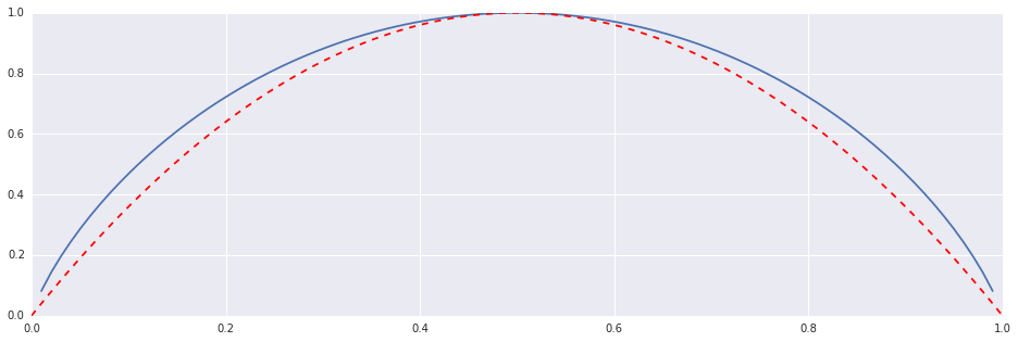
So calculating the entropy associated with a given value of $p$ is simple. But the converse is not as simple. I don’t know how to analytically solve this, but numerically I do: $H(p)$ is parabola-ish, so it can be reasonably approximated by the quadratic function whose roots are 0 and 1, and its vertex’s height is 1, i.e. $4p(1-p)$:

In [3]:

H = lambda p: -p*numpy.log2(p)-(1-p)*numpy.log2(1-p)
F = lambda p: 4.0*p*(1-p)
p = numpy.linspace(0,1,100)
plt.plot(p, H(p))
plt.plot(p, F(p), '--r')

Out [3]:

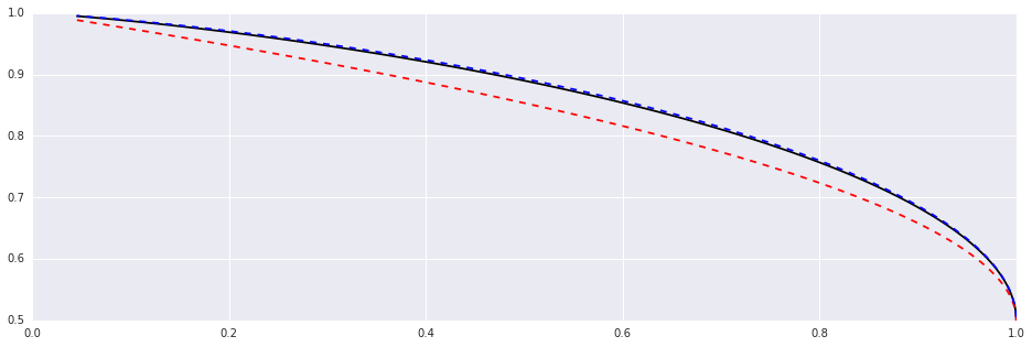
So to a first approximation, $H=4p(1-p) \Rightarrow p=\frac{1}{2}\sqrt{1-H}$. It is crude, but it doesn’t matter: since $H’(p)=-\log_2(\frac{p}{1-p})$ we can satisfactorily improve this approximation by one Newton’s iteration (for solving $H+p\log_2(p)+(1-p)\log_2(1-p)=0$):

In [4]:

def inverse_entropy_raw(H):
    return 0.5*(1.0+numpy.sqrt(1.0-H))  # H(p) ~ 4.0p(1-p)

def inverse_entropy(H):
    p = inverse_entropy_raw(H)
    f = H+p*numpy.log2(p)+(1-p)*numpy.log2(1-p)    
    ft = numpy.log2(p/(1.0-p))
    return p - f/ft # Newton's iteration

p = numpy.linspace(0.5,1.0,100)
plt.plot(H(p), p, 'k')
plt.plot(H(p), inverse_entropy_raw(H(p)), '--r')
plt.plot(H(p), inverse_entropy(H(p)), '--b')

Out [4]:

And now we have a solution:

In [5]:

def random_bitstream3(size_in_bytes, entropy):
    p = inverse_entropy(entropy)
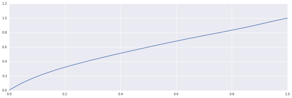
    return numpy.packbits(numpy.random.choice((0,1), size=size_in_bytes*8, p=(p, 1-p))).tobytes()

As a sanity check, let’s verify that the requested entropy indeed roughly corresponds to the “compression rate” of the generated data (this is expected for large data, since the bits are generated independently):

In [6]:

def estimate_compression_rate(entropy, bytes=1024*128, iters=5):
    compression_rate = lambda blob: len(zlib.compress(blob, 1))/(len(blob)+0.0)
    return numpy.mean([compression_rate(random_bitstream3(bytes, entropy)) for i in xrange(iters)])

entropies = numpy.linspace(0.001, 0.999, 25)
compression_rates = numpy.array([estimate_compression_rate(entropy, iters=3) for entropy in entropies])
plt.plot(entropies, compression_rates)

Out [6]:

So far so good, with just one issue: efficiency. To generate 1MB of data, it requires 64MB of RAM, and considering the fact that it’s going to be used to generate many gigabytes of data, it’s very slow:

In [7]:

%timeit -n10 random_bitstream3(1024*1024, 0.5)

Out [7]:

10 loops, best of 3: 311 ms per loop

That’s over 5 minutes per gigabyte.

As a reference, compare it to the non-parametric version:

In [8]:

%timeit -n10 random_bitstream1(1024*1024)

Out [8]:

10 loops, best of 3: 1.54 ms per loop

The memory issue is solvable by generating streams in pieces, but the speed seems to be a fundamental problem of drawing 1 bit at a time.

Thinking straightforwardly again, it seems reasonable the draw chunks instead of bits. Consider, for example, drawing 1 byte at a time. Since each random byte is a sequence of 8 random bits, the number of ‘0’s is binomially distributed $B(8,p)$. So iterating the following 2 steps, achieves the same distribution of bits:

1. Draw N from $B(8,p)$.
2. Draw a Byte with exactly $N$ ‘0’s (uniformly from the $\binom{8}{N}$ admissible bytes).

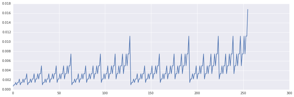
This can be done faster and cleaner in just 1 step, by pre-calculating the probability of drawing each byte, and draw directly from the corresponding probability vector.

In [9]:

def precalculate_probabilities(p, bits):
    weights = numpy.array([scipy.special.binom(bits, i)*(p**i)*((1-p)**(bits-i)) for i in xrange(bits+1)])
    values = numpy.arange(2**bits, dtype=numpy.ubyte)
    probabilities = numpy.zeros(values.shape)
    for i, v in enumerate(values):
        probabilities[i] = weights[gmpy.popcount(i)]/(scipy.special.binom(bits, gmpy.popcount(i))+0.0)
    return values, probabilities
    
values, probabilities = precalculate_probabilities(0.6, 8)
plt.plot(values, probabilities)

Out [9]:

In [10]:

class RandomBitstreams(object):
    def __init__(self, p, chunk_bytes=1, seed=None):
        if seed:        
            numpy.random.seed(seed)
        self._chunk_bytes = chunk_bytes
        self._values, self._probabilities = precalculate_probabilities(p, 8*chunk_bytes)
        
    def bitstream(self, size_in_bytes, seed=None):
        if seed:        
            numpy.random.seed(seed)            
        return numpy.random.choice(self._values, size=size_in_bytes/self._chunk_bytes, p=self._probabilities)
    
generator = RandomBitstreams(0.5)

In [11]:

%timeit -n10 generator.bitstream(1024*1024)

Out [11]:

10 loops, best of 3: 82.5 ms per loop

This is ~300%-400% faster, but not fast enough.

A major improvement can be done by taking inspiration from cryptographic ciphers. The possibilities are numerous, and here are two such schemes. The first is directly analogous to block ciphers, and the second is more combinatorial in nature.

Bitwise operations are central to both ideas. Recall: $\land$ is “$\mathrm{and}$”, $\lor$ is “$\mathrm{or}$” and $\oplus$ is “$\mathrm{xor}$”.

As we have seen, it is possible to generate random bitstreams rather fast (e.g. using numpy.random.bytes). The first idea is to do just that, but then modify the stream’s entropy by some bitwise operations relying on the following observation: Let $C$ be a random bitstream taken from $B(n,p)$, and denote $p(C)=p$.

Then $p(C_1\land C_2)=p(C_1)p(C_2)$ and $p(C_1\lor C_2)=1-(1-p(C_1))(1-p(C_2))$.

If we’re given a bitstream $M$ of length $n$ (with $p(M)\ge\frac{1}{2}$), and have a “key” $K$ with the same length, then $M\land K$ is a new bitstream of length $n$ with an increased entropy, $M\lor K$ is a new bitstream of length $n$ with a decreased entropy, and the change of entropy is controllable by choosing $p(K)$.

We can obtain a new bitstream $M’$ with $p(M’)>\frac{1}{2}$ by taking $M’:=M\lor K$ where $p(M’)=1-(1-p(M))(1-p(K))\Rightarrow p(K)=1-\frac{1-p(M’)}{1-p(M)}$, and obtain a new bitstream $M’$ with $p(M’)<\frac{1}{2}$ by taking $M’:=M\land K$ with $p(K))=\frac{p(M’)}{p(M)}$ (as expected, “or”ing requires $p(M)\le p(M’)$ and “and”ing requires $p(M)\ge p(M’)$, and in our setting $p(M)=\frac{1}{2}$ - so both are equally valid).

Of course, the simplistic method of holding one such key and applying it block- wise on $M_1,… ,M_m$ to get a new bitstream of length $nm$ won’t work well. The resulting entropy would be right, but the bit-pattern of $K$ will induce dependencies over the bits of the new bitstream, that dictionary coders could exploit.

A plausible solution is to choose $K$ randomly from a pre-generated suitable collection (generating $K$ ad-hocly would defeat the purpose of shortening execution time). Since we’re interested in the entropy, not probability, we may assume $p(M’)\ge\frac{1}{2}$ (or otherwise $\mathrm{not}$ the result).

As a final improvement, I suggest to use both $\land$ and $\lor$ at each step (e.g. first $\land$, then $\lor$). The additional overhead of performing 2 bitwise operations instead of 1 per block is negligible, and it allows us to get the same pseudo randomality we previously achieved using $r$ keys, by using just $\sqrt{r}$ keys. Specifically, if $p(M’)\ge\frac{1}{2}$ we may do this with any arbitrarily choice of $p(K_\mathrm{and})$ and $p(K_\mathrm{or})=1-\frac{1-p(M’)}{1-\frac{1}{2}p(K_\mathrm{and})}$.

In [12]:

def andor_perturbation_probabilities(p_target, p_and=0.5):
    p_or = 1-(1-p_target)/(1-p_and/2.0)
    return p_and, p_or


class AndOrPerturbator(object):
    def __init__(self, p, block_bytes, keys):
        p_and, p_or = andor_perturbation_probabilities(p)

        gen_or = RandomBitstreams(p_or)
        gen_and = RandomBitstreams(p_and)
        
        k = int(numpy.ceil(numpy.sqrt(keys)))
        self._orKs = [gen_or.bitstream(block_bytes) for i in xrange(k)]
        self._andKs = [gen_and.bitstream(block_bytes) for i in xrange(k)]
        self._block_bytes = block_bytes

    def keys_count(self):
        return len(self._orKs)
        
    def block_size(self):
        return self._block_bytes
    
    def perturbe_block(self, M, i, j):        
        return numpy.bitwise_or(numpy.bitwise_and(M, self._andKs[i]), self._orKs[j])
    

def perturbe(M, perturbator):
    k = perturbator.keys_count()
    block_bytes = perturbator.block_size()

    length = len(M)
    count = int(numpy.ceil(length/(block_bytes+0.0)))
    M = numpy.pad(numpy.fromstring(M, dtype=numpy.ubyte), pad_width=(0, block_bytes*count-length), mode='edge')
        
    perturbe_block = lambda block: perturbator.perturbe_block(block, numpy.random.randint(k), numpy.random.randint(k))
    Mtag = numpy.hstack([perturbe_block(M[i*block_bytes:(i+1)*block_bytes]) for i in xrange(count)])
    return Mtag[:length]

perturbator = AndOrPerturbator(0.67, 8*1024, 128)

In [13]:

%timeit -n10 perturbe(numpy.random.bytes(1024*1024), perturbator)

Out [13]:

10 loops, best of 3: 4.71 ms per loop

That’s an improvement of ~6000%-7000% from the initial algorithm, but it’s still slower than simply generating random bytes. Can we further approach the performance of numpy.random.bytes, while still controlling the entropy?

Yes we can. The key is to switch from perturbation to generation. Instead of using a pair of “keys” to perturbate external data, we will treat the keys as “building blocks” and combine them to generate new blocks, with the required entropy. The large combinatorial space of building-blocks can make the likelihood of exploitable dependencies arbitrarily low.

This is really simple, and amounts to nothing more than this observation: $p(C_1\oplus C_2)=p(C_1)(1-p(C_2))+p(C_2)(1-p(C_1))$ (based on the slogan “xor rewards disagreements”).

Now all that is left is to generate 2 pools of “building blocks” for any given $p(M’)$. The first pool may contain blocks whose entropy is maximal, and independent of $p(M’)$ (so they can be generated quickly, and possibly in advance - an optimization that is not in the code below), and the second pool contains blocks whose entropy is chosen so that $p(C_1\oplus C_2)=p(M’)$ where $C_1$ is taken from the first pool, and $C_2$ from the second.

In [14]:

def xor_adjoint_probabilities(p):
    calc = lambda p: ((1-p)/2.0, (1.5*p-0.5)/p)
    if p >= 0.5:
        return calc(p)
    else:
        x, y = calc(1-p)
        return x, 1-y

class CombinatorialGenerator(object):
    def __init__(self, p, block_bytes, pool_size):
        pH, qH = xor_adjoint_probabilities(p)

        gen_p = RandomBitstreams(pH)
        gen_q = RandomBitstreams(qH)
        
        components = int(numpy.ceil(numpy.sqrt(pool_size)))
        self._ps = [gen_p.bitstream(block_bytes) for i in xrange(components)]
        self._qs = [gen_q.bitstream(block_bytes) for i in xrange(components)]
        self._block_bytes = block_bytes
        
    def components(self):
        return len(self._ps)

    def block_size(self):
        return self._block_bytes
    
    def block(self, i, j):
        return numpy.bitwise_xor(self._ps[i], self._qs[j])
    

def combine(bytes, combiner):
    k = combiner.components()
    block_bytes = combiner.block_size()
    count = int(numpy.ceil(bytes/(block_bytes+0.0)))   
    return numpy.hstack([combiner.block(numpy.random.randint(k), numpy.random.randint(k)) for i in xrange(count)])[:bytes]


combiner = CombinatorialGenerator(0.74, 8*1024, 1024*1024)

In [15]:

%timeit -n10 combine(1024*1024, combiner)

Out [15]:

10 loops, best of 3: 1.6 ms per loop

The larger the blocks, the faster this generator works. The price is a reduced pseudo randomality for long bitstreams. But as long as the bitstream size (in bytes) is less than “pool_size times block_bytes” this is not an issue for the purpose of testing compression, and it’s easy (and quick) to reinitialize the generator once it’s exhausted.

We conclude with a sanity check:

In [16]:

compression_rate = lambda blob: len(zlib.compress(blob, 9))/(len(blob)+0.0)

combiner = CombinatorialGenerator(0.5, 1024, 1024)
x = numpy.hstack([combiner.block(i,j) for i,j in itertools.product(xrange(32), xrange(32))]).tobytes()

print 'Exhausted Combiner - Compression rate: ', compression_rate(x)
print 'Random Bitstream   - Compression rate: ', compression_rate(numpy.random.bytes(1024*1024))

Out [16]:

Exhausted Combiner - Compression rate:  1.00031089783
Random Bitstream   - Compression rate:  1.00031089783